Interior Reconstruction under Occlusion and Clutter, based on the 3D Hough Transform

Transcription

1 School of Engineering and Science Bachelor s Thesis Interior Reconstruction under Occlusion and Clutter, based on the 3D Hough Remus-Claudiu Dumitru May 2012 First supervisor: Prof. Dr. Andreas Nüchter

2

3 Abstract Laser scanners are often used nowadays to create accurate 3D models of buildings for civil engineering purposes, but the process is currently done manually and proves to be time consuming and error-prone [4]. Therefore, the need to characterize and quantify such complex environments arises, posing challenges for data analysis. This thesis presents a method to reliably detect planes in 3D point clouds [9], based on which the scene will be reconstructed at a high architectural level by removing clutter and foreground data. The implemented software will detect openings, such as windows and doors, in order to complete the architectural model. In addition, it will label detected planes accordingly to floor, ceiling or wall. Extracting such components from the 3D data proves to be difficult due to various reasons such as boundary detection of openings. Occlusions need to be distinguished from actual openings and occupied regions in openings need to be disregarded completely. Methods for overcoming such impediments are also presented here, aiming to overcome drawbacks imposed by missing data by filling in occluded regions and accurately detecting openings.

4 Acknowledgments I would like to express my deepest gratitude to my supervisor, Prof.Dr. Andreas Nüchter, for his constant support during the entire duration of this guided research. Furthermore, I would also like to thank Dorit Borrmann and Jan Elseberg for their help regarding various technical difficulties and for acquiring the scans.

5 Contents 1 Introduction Problem Definition Goal Possible Impediments Scientific Contribution Motivation Semantics and Semantic Mapping in 3D Point Clouds State of the Art Current Approaches Plane Detection in Point Clouds Interior Reconstruction under Occlusion and Clutter The Software Environment The 3D Toolkit Scan Registration Component Visualization Plane Detection Other Software Methodology Preliminary Assumptions The Point Cloud Processing Pipeline The Interior Reconstruction Pipeline Scene Initialization Wall Detection Occlusion Labeling Opening Detection Occlusion Reconstruction Experiments and Results Environment General Results v

6 6 Future Work Interchangeable components Extending the pipeline Additional tests Conclusion 51 vi

7 Chapter 1 Introduction The laser scanner has been one of the most used sensors in robotics, and so far many algorithms for manipulating 3D point cloud data exist, but very few of them tackle the idea of semantics, the idea of what do these point clouds actually represent. One example of such algorithm that does not tackle the idea of semantics is the 6D Simultaneous Mapping and Localization Algorithm such as the one used for the DARPA Urban Challenge [1]. On the other hand, some advances have been made in the field of object recognition by the people at Willow Garage using their famous robot, the PR2, and their Point Cloud Library [15]. Jacobs University Bremen also has made some advances in the field through its Robotics Group at the ICRA Robot Challenge by placing second in this contest [11]. But these are just a few minute examples of tackling the idea of semantics in point cloud data. This research proposes the analysis of 3D point cloud data on a larger scale. It will focus on interior reconstruction from 3D point cloud data and the main tool of achieving this goal will be the 3D Hough aiding in the efficient extraction of planes. The proposed software environment is the 3D Toolkit [18] which already contains an efficient plane extraction from 3D point clouds feature developed by Prof. Dr. Andreas Nüchter et al. at Jacobs University Bremen [9]. Furthermore, Adan and Huber state [4] that there have been attempts to automate interior and exterior reconstruction, but most of these attempts have tried to create realistic models, instead of trying to achieve a geometrically accurate one. Also they state that other approaches exist, such as image and video-based approaches, but these are not accurate enough, with the exception of Manhattan world stereo, which shows some promise. Now that laser scanner technology has progressed researchers have started to show more interest in it. But with this technology new problems arise, such as occlusions and cluttering. Their paper proposes an efficient way on how to reconstruct the scene and how to fill in the missing information created by occlusion and cluttering. All in all, this research proposes to extend the work of Nüchter [9] and that of Adan and Huber [4, 5] by combining Nüchter s approach of plane extraction and Adan s and Huber s approach to 3D reconstruction of interiors under occlusion and clutter, in order to reconstruct the scene at a high architectural level. 1

8 2 CHAPTER 1. INTRODUCTION 1.1 Problem Definition Goal The goal is to reconstruct the scene, here a point cloud scan of the interior of a building, at high architectural level. The main idea is that planes will be detected using the 3D Hough already implemented in the 3D Toolkit [9], and using these planes, the developed software will decide if the plane actually defines a wall of the interior. The Hough is well known to be used in the processing of 2D data for detecting lines and circles [9], but Nüchter noticed the potential of it in 3D in order to detect planes in point clouds. This will prove to be a very powerful tool in this proposed research as interiors mostly comprise of planar surfaces, with the exception of certain modern architectural approaches such as curved walls or textured surfaces, but such impediments will be discussed in the next section. Figure 1.1: Contribution. The research provided by Nüchter et al. mainly focuses on various implementations of the 3D Hough. All these implementations are included in the 3D Toolkit and will be at our disposal during the proposed research. In the end, only the Randomized Hough (RHT) will be used since as the paper concludes, it performs the best. On the other hand, besides determining the planes that resemble the walls of an interior, we must also determine what is an occlusion and what is actually empty space, in order to accurately determine the position of openings such as windows and doors. Thus, in this case missing information drastically affects the outcome of the reconstruction. Interpreting an occlusion as an opening is certainly not desired. Adan and Huber propose a few simple steps in overcoming impediments such as missing information [4, 5]: a. Wall detection - in this research we propose to use the plane detection already implemented in 3DTK [9] b. Occlusion labeling - for each wall surface, ray-tracing is used to determine which surface regions are sensed, which are occluded, and which are empty space [4]

9 1.1. PROBLEM DEFINITION 3 c. Opening Detection - a learning-based method is used to recognize and model openings in the surface based on the occlusion labeling [4] d. Occlusion Reconstruction - occluded regions not within an opening are reconstructed using a hole-filling algorithm [4] Therefore, the pipeline described above will be used to fill in the missing information in order to accurately detect the openings. Obviously it is expected that better results will be achieved for simple, normal buildings, and the less occlusions there are, e.g. the less furniture there is, and the simpler the structure of the building is, the better the results will be. In the end, our aim is to combine these two methods and yield a piece of software (part of 3DTK) that will be able to take as input a point cloud of an interior and in the end output a geometrically accurate model of that interior, removing cluttering and foreground data, filling in the gaps, placing walls and labeling them appropriately, distinguishing between wall, ceiling, floor etc., detecting openings and placing windows in the appropriate location with correct size; we will ignore the shape for now and assume all windows are rectangular Possible Impediments It is clear that the outcome of the research will closely depend on the performance of the plane extraction algorithm and on the quality of the scans taken. To begin with, we have taken a few scans around the interior of the Research 1 building at Jacobs University Bremen using a RIEGL VZ-400 laser scanner. The scans prove to be very accurate, and multiple scans can be taken and put together using the scan registration feature of the 3DTK. How accurately the plane extraction algorithm is will drastically affect the outcome of the proposed research. Also, the performance of the pipeline proposed in [4, 5] is another factor, but experimental results of the researchers has proven that overall their approaches provide valid results. Putting performance issues aside and focusing on various details of the interiors, it must be added that variables such as the following will affect the outcome: overall shape of the interior number of walls (4 expected, typical room) wall texture (affects plane detection) unexpected architectural shapes (e.g. The Gates Building at CMU) shape of the openings (possible round windows) opening transparency mirrors, or glass objects window frame thickness (may lead into thinking window is not an opening) irregularities in the openings (e.g. window mounted objects) furniture (adding to the number of occlusions) number of scans taken (the more scans we have, the better outcome, after registration) resolution of the scans The list is easily extensible, and these are some of the few important features that may simply lead the algorithm into taking an invalid decision.

10 4 CHAPTER 1. INTRODUCTION 1.2 Scientific Contribution As [4] states, there is a large body of research on reconstruction of building interiors and exteriors using laser scanners such as [6 8, 12, 14, 16, 20, 21, 24, 25], but much of this work focuses on creating a visually realistic model, rather than a geometrically correct one. Thus our work will aim at filling in these gaps, and provide a software implementation that constructs an accurate architectural model from a geometrical point of view. 1.3 Motivation What drives us into pursuing this research is the small number of contributions to this field and the need for such a software to exist. There is an increasing need for rapid characterization and quantification of complex environments driven by important areas such as industrial automation, architecture, agriculture, and the construction or maintenance of tunnels and mines. We mostly focus on the needs coming from architecture, engineering and construction (AEC) [4], such as building renovation cultural heritage preservation and facility management. Such models are usually, manually reconstructed and prove to be labor-intensive and tedious processes. As a consequence, the need for such a software package Semantics and Semantic Mapping in 3D Point Clouds A 3D point cloud is simply a collection of 3D coordinates, they posses no meaning, and no interpretation. Using various visualization software, these point clouds can easily be interpreted by a person in the sense that a person is able to determine if, for example, a silhouette belongs to person, or if it is the silhouette of a tree. Furthermore, points may have a certain color mapping, be it a color mapping representing surface temperature, or each point is mapped to its visible light color, making things much easier for a human to interpret the point clouds, but for a machine to automatically determine semantically what a collection of points represent is no easy task. Recently, certain advancements have been made in this field helping us to cross the border into semantics and semantic mapping and the first step is to extract shapes, even the most basic ones, such as planes. Similar techniques are being used to extract more complicated shapes, but this is not the matter of this research. Determining if a collection of points from a 3D point cloud form a plane is slightly more related to semantics. We propose to determine if such a plane is actually a wall inside a room, the floor, or the ceiling. Furthermore, these planes will contain missing information, such as gaps, and the aim is to accurately determine, from a semantic point of view, if these gaps represent occlusions or if they represent actual openings in the walls, thus determining if they are windows or doors. All in all, this is what we mean by semantics in the case of 3D point clouds, attributing a meaning to a set of points, an interpretation us humans are able to understand.

11 Chapter 2 State of the Art As mentioned in the previous chapter, there is a large body of research done in this field, but it mainly focuses on creating an aesthetically accurate model, rather than a geometrically accurate one [4]. Papers that approach the issue from such a point of view are [6 8,12,14,16,20,21,24,25], which in contrast to our goal, they only attempt to construct a model of the interior and exterior of a building by conserving aesthetic details and not focusing on the geometrical truth and the semantics of the 3D data. 2.1 Current Approaches So far, we have mentioned two main approaches that will be used for this research. One involves the plane extraction, and this relates to the work of Nüchter, and the other one involves the removal of cluttering and foreground data, and this involves the work of Adan and Huber. We will implement our own approach by merging these two together and further improving and extending them, in addition, integrating the developed software with the 3DTK Plane Detection in Point Clouds The basis of the plane detection algorithm is the patent published by Paul Hough in 1962 [17]. This is the main approach behind [9], with various changes and approaches to it. The Hough has had many uses for the case of 2D in extractions of various features, mainly lines and circles, but Nüchter, and also Adan and Huber proposed to use it on 3D data. Before getting into more details regarding different implementations of the 3D Hough, let us first present the general idea behind the method. Nüchter [9] defines the Hough as being a method for detecting parametrized objects, typically used for lines and circles. Although the original application of the Hough was on pixel images, this is not a necessity. In the current scenario we are dealing with uncategorized 3D point cloud data as input, and the output consists of parametrized planes. The common representation for a plane is the signed distance ρ to the origin of the coordinate system, and the slopes m x and m y in direction of the x and y axis. All in all, we can parametrize a plane as z = m x x+m y y +ρ. In order to avoid problems caused by infinite slopes during the representation of vertical planes, 5

12 6 CHAPTER 2. STATE OF THE ART the Hesse Normal Form is used, a method that uses normal vectors. Consequently, the plane is thereby given by a point p on the plane, and the normal vector n that is perpendicular to the plane, and the distance ρ to the origin. Therefore, the parametrization of the plane becomes: ρ = p n = p x n x + p y n y + p z n z (2.1) In order to find points in a point set, we must calculate the Hough for each point. Given such a point p in Cartesian coordinates, we must determine all the planes the point lies on. Marking such points in the Hough Space will lead to a 3D sinusoid curve, as shown in Figure 2.1. Figure 2.1: ation of three points from R 3 into Hough Space (θ, ϕ, ρ). The intersection of the curve (marked in black) depicts the plane spanned by the three points [9]. The intersections of two curves in Hough Space denote the set of all possible planes rotated around the lines defined by two points. Consequently, the intersection of three curves in Hough Space will correspond to the polar coordinates defining the plane spanned by the three points [9]. Now that we have discussed the general approach of the Hough applied to 3D data, let us continue with the various Hough methods used. Nüchter [9] describes various ways of extracting planes via different Hough methods such as: a. Randomized Hough - rht b. Standardized Hough - sht c. Probabilistic Hough - pht

13 2.1. CURRENT APPROACHES 7 d. Progressive Probabilistic Hough - ppht e. Adaptive Probabilistic Hough - apht f. Randomized Sample Consensus (RANSAC) - ran All these methods are already implemented in the 3DTK [18] and are available via the -p flag on the command line when using the planes executable. The possible choices are the ones marked above in bold text. Among all these methods, the Randomized Hough is the one of most interest to us as [9] concludes that it has exceptional performance as far as runtime is concerned. For convenience, we present the algorithm for RHT: Algorithm 1 Randomized Hough (RHT) [9] 1: while still enough points in point set P do 2: randomly pick points p 1, p 2, p 3 from the set of points P 3: if p 1, p 2, p 3 fulfill the distance criterion then 4: calculate plane (θ, ϕ, ρ) spanned by p 1, p 2, p 3 5: increment cell A(θ, ϕ, ρ) in the accumulator space 6: if the counter A(θ, ϕ, ρ) equals the threshold t then 7: (θ, ϕ, ρ) parametrize the detected plane 8: delete all points close to (θ, ϕ, ρ) from P 9: reset the accumulator 10: end if 11: else 12: continue 13: end if 14: end while The basis of the Randomized Hough algorithm is the article A new Curve Detection Method: Randomized Hough (RHT) [26] which was initially intended for the processing of 2D data. Also worth mentioning is the paper Fast Plane Detection and Polygonalization in noisy 3D Range Images [19] which helped in the efficient detection and polygonalization of the planes, thus making it possible to efficiently construct the planes in OpenGL using polygons and displaying them. Regarding the Standard Hough, Nüchter [9] mentions that due to its high computation time, it is rather impractical, especially for real-time applications. Nevertheless, we present Algorithm 2, to be used as a reference. We will not present all the algorithms in detail (see [9] for all implementations); instead we will compile all the distinctive characteristics of the Hough methods into Table 2.1. Notice that in the steps mentioned to remove clutter and replace missing data we talk about voxels and not about points from the point clouds. This is where [5] comes into play. The paper first introduces the notion of building information model (BIM), and defines it as being the 3D model of a building. As previously mentioned, typically BIM s are made manually by people.

14 8 CHAPTER 2. STATE OF THE ART Algorithm 2 Standard Hough (SHT) [9] 1: for all points in p i in point set P do 2: for all cells (θ, ϕ, ρ) in accumulator A do 3: if point p i lies on the plane defined by (θ, ϕ, ρ) then 4: increment cell A(θ, ϕ, ρ) 5: end if 6: end for 7: end for 8: search for the most prominent cells in the accumulator that define the detected planes in P SHT PHT PPHT APHT RHT complete / deterministic stopping rule adaptive stopping rule delete detected planes from point set touch only one cell per iteration easy to implement Table 2.1: Distinctive characteristics of Hough methods We desire to automate this process and save precious man hours from being lost. Initially [5] introduces the method on how to extract the planes, but as we have mentioned before the 3DTK implementation will be used [9]. Nevertheless, this part may still prove to be important for our cause as it explains how to discretize the space and make the algorithm more efficient, as Occlusion Labeling, Opening Detection, and Occlusion Reconstruction, all operate on voxels. Adan and Huber propose the following steps to discretize the scene and extract the planes [5]: a. Voxelization We discretize the input point cloud into a uniformly spaced 3D grid data structure (voxel space). This tends to reduce data in dense areas, and keep data in sparse areas, this overall having little effect on the outcome, except for improving runtime performance. b. Patch Detection Planar patches are extracted from the voxel space by implementing a region growing algorithm to connect nearby points that present similar surface normals and that are well described by a planar model. c. Patch Classification Modeled patches are classified according to the following labels: wall, ceiling, floor, or clutter using a context-based algorithm that is modeled using a conditional random field (CRF). This may prove to be useful, since the 3DTK implementation simply extracts the planes and does not classify them. Also helps detecting clutter, aiding us in removing it later on.

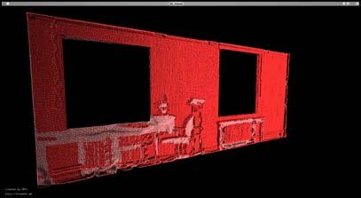
15 2.1. CURRENT APPROACHES 9 d. Patch Intersection The boundaries of the patches are cleaned up by intersecting the adjacent patches and the patches labeled as cluttered are simply removed. In the end, the steps above will yield a compact model of the walls, floor, and ceiling of a room, and each patch is labeled accordingly Interior Reconstruction under Occlusion and Clutter Previously, we have discussed various difficulties we may encounter in 3D laser scans. Our research is mostly affected by cluttering and foreground data. Laser scanners do not have a perfect 180 vertical field of view, therefore there will be missing information in the point cloud above and below the scanner. Moreover, occlusions also make our task more difficult. Our aim is to extract the right information despite these setbacks. Papers [4,5] propose a way of reconstructing interiors from 3D point clouds and manage to find a way to overcome obstacles such as the ones mentioned above by the use of supervised learning. Adan and Huber propose the following steps [4, 5]: a. Wall Detection This has already been discussed in the previous section. We will use approaches mentioned in [9] to detect the planes and use approaches mentioned in [5] to classify each plane and decide whether it is a ceiling, floor or wall. Figure 2.2: Scan of an empty office with planes detected using RHT [9] b. Occlusion Labeling In each step, each voxel in each surface is assigned one of three possible labels: occupied, empty or occluded. The labeling takes place for each scanning position that has sight of the surface at hand and then the information is merged together into a unified representation. The labeling as empty or occupied is done by deciding whether a surface was detected at that

16 10 CHAPTER 2. STATE OF THE ART location or not. At this point distinguishing between a voxel that is empty or occluded is not quite possible. This problem is addressed by performing ray-tracing to explicitly decide between occluded or empty. Figure 2.3: Occlusion labeling [4]. (a) Reflectance image from one of five scans used to model the wall. (b) Ray-tracing is used to label occlusion regions on the surface. (c) Labels from multiple laser scans are integrated into a single representation. (d-e) A high resolution labeling (e) is inferred using a region-growing algorithm based on seeds from the low resolution data (d). c. Opening Detection The difficulty in deciding whether a portion of the surface is empty is difficult since parts of this opening may be labeled as occupied, e.g. a window mounted fan or the window frame could be very thick. The algorithm proposed, which detects rectangular openings, uses features derived from labels and depth edges in the data to learn a model of the size, shape, and location of openings using a Support Vector Machine (SVM) classifier. Figure 2.4: Opening detection [4]. (a) Reflectance image of a wall surface. (b) Corresponding depth image. (c) Detected lines overlaid on edge image. (d) Openings detected by the SVM-based detector, with each cluster of openings in a different color. (e) Prototype openings after clustering, superimposed on I F. (f) Final labeling with openings masked out.

17 2.1. CURRENT APPROACHES 11 d. Occlusion Reconstruction Once the openings are determined, int the end all we need to do is fill in the surface where we have voxels labeled as occluded. The paper proposes to use the gap-filling algorithm described by [23]. Their idea is to acquire a 2D projection of the 3D data while also storing depth information. Then 2D image restoration algorithms are being used in order to fill in the gaps and then the inverse is being applied, more clearly, the 2D projection is transformed again into a 3D representation of the data. In more technical words, the paper proposes a 3D extension of the Markov Random Field inpainting algorithm which is described in [22]. Figure 2.5: Occlusion reconstruction [4]. Two examples showing the surface before (a, c) and after (b, d) reconstruction. As mentioned numerous times throughout this paper, there is a large body of papers tackling similar issues, but from an aesthetic point of view. For example take papers [6 8] which focus on the exterior of buildings, and [12] which focuses on interior reconstruction, but does not take into consideration openings. (a) Exterior (b) Interior Figure 2.6: Interior and exterior aesthetic models [6 8, 12]. On the topic of aesthetic reconstruction of building exteriors are also [14] and [16].

18 12 CHAPTER 2. STATE OF THE ART Figure 2.7: Photograph of two buildings from the University of Freiburg (left), building model (right) [16] An interesting approach to exterior reconstruction is [20]. It seems that the goal is to semantically extract the features of the building, but the source consists of 2D images and not 3D point clouds. Nevertheless, the approach is capable of detecting windows. Figure 2.8: Extracting significant lines from an image [20] Among the approaches on exterior reconstruction, the one most related to our research is [21]. This in one of the papers that tries to semantically detect features of a building facade. Figure 2.9: Point cloud of a facade and reconstruction result [21]

19 Chapter 3 The Software Environment As mentioned in the previous chapters, the software environment of choice is 3DTK - The 3D Toolkit, developed by Prof. Dr. Andreas Nüchter from Jacobs University Bremen and Prof. Dr. Kai Lingemann from The University of Osnabrück. 3.1 The 3D Toolkit The toolkit provides algorithms and methods to process 3D point clouds. It includes automatic high-accurate registration (6D SLAM), and other tools like a fast 3D viewer, plane extraction etc. Full details on how to acquire the software can be found at [18]. Moreover, the 3DTK is capable of handling various file formats Scan Registration The process by which scans are merged into one coordinate system is called registration and this is what the slam6d component does. There are two types of algorithms that slam6d can use [18]: a. ICP Matching: Also known as sequential matching, this type of matching goes over the scans sequentially. It takes two scans at a time. b. Global Matching: This type of matching can process multiple of scans at one time and the sequence of the scans does not matter. When Global matching is used, a second parameter must be specified. By default, the slam6d component uses the sequential matching. An example of the command for the slam6d component using some specification parameters will be: slam6d s 1 e 60 dat So the slam6d component takes the scans as inputs and generates *.frames files as output. 13

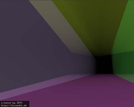
20 14 CHAPTER 3. THE SOFTWARE ENVIRONMENT Component Visualization In order to view registered point clouds, or even simple scans and extracted planes the 3DTK contains a viewer component called show. An example of the command for the show component using some specification parameters will be: show s 1 e 76 m 3000 dat In order to easily visualize the data, the show component presents a user friendly graphical user interface: Figure 3.1: 3DTK show GUI The GUI offers controls to alter appearance and navigation. For each, there is an appropriate window containing various options the user can set. For further details please consult the full description on how to use the software [18] Plane Detection The most important component of the 3DTK for our proposed research is the plane extraction component. In order to extract planes, this component is first called on the data set. This, in turn, will create a planes folder, containing information regarding each detected plane in *.3d files and a planes.list file, containing the list of the detected planes. Then the point cloud can be displayed concurrently with the detected planes using the show component.

21 3.1. THE 3D TOOLKIT 15 (a) Including points (b) Only planes Figure 3.2: Plane extraction, first view (a) Including points (b) Only planes Figure 3.3: Plane extraction, second view

22 16 CHAPTER 3. THE SOFTWARE ENVIRONMENT 3.2 Other Software The following is a list of software programs used during the course of this guided research: a. Kubuntu LTS the Operating System of choice b. 3DTK the 3D data manipulation environment c. C++ the programming language of choice d. CGAL C++ library used to compute the concave hull e. OpenCV C++ library machine learning and image processing algorithms provided f. Eigen C++ library linear algebra g. Eclipse CDT the IDE of choice h. Kile integrated L A TEXeditor i. L A TEX the document preparation system j. Dia diagram creator k. GanttProject GANTT chart creator l. Subversion version control software

23 Chapter 4 Methodology 4.1 Preliminary Assumptions First and foremost, a set of assumptions must be clearly defined before any implementation. This set of assumptions only aids in simplifying the task and ensuring good, accurate results. In other words, the aim of these assumptions is to avoid any ambiguous architectural components frequently found in modern buildings, which present odd shapes and tend to use some materials, like glass, in excess. Furthermore, we ensure that the environment is properly set up, in order for components to work properly. Among such assumptions we enumerate: all surfaces, such as walls, floors and ceilings are flat and have regular shapes, to ensure that the plane detection algorithm [9] accurately detects these surfaces which are crucial for the remaining steps of our approach; in addition, we also assume that all walls are vertical, floor and ceiling are horizontal, and only a single room is contained in a scan all openings are rectangular, and may present irregularities such as window mounted objects which will appear as occupied space in our labeling; furthermore, if the opening is not rectangular, but displays features close to a rectangular window, it will be detected by the Support Vector Machine [3], but it will be represented as a rectangular opening the amount of occlusion in the point cloud is within acceptable margins, meaning that it allows the wall detection algorithm to detect all the walls; if a wall is completely occluded it is impossible to detect for performance reasons, it is recommended that a point cloud reduction is applied beforehand especially if running on a slower machine with low memory; moreover, if such a reduction is performed, it must be ensured that the points are randomly selected from the occupied voxels, such that the points in a horizontal slice are not perfectly aligned; the reason for this is that the plane detection algorithm will detect a lot of false planes, as it will find many coplanar points stacked closely together and detect them as a plane in order to further improve the overall runtime, we make use of some configuration values, such as the minimum and maximum allowed size of an opening, or minimum Empty area 17

24 18 CHAPTER 4. METHODOLOGY for a candidate to count as an opening; these values are only prior estimates of the scene to be processed, and help us avoid redundant computation; further details will be given in the following sections 4.2 The Point Cloud Processing Pipeline The main focus of this research is to harness the potential of the 3D Hough and utilize it in order to achieve a geometrically accurate model of an interior. Before we can run the plane detection algorithm, the 3D data needs to be pre-processed. Firs and foremost, 3D point clouds require a lot of memory, a lot more than a typical personal computer has, thus scan reduction needs to be applied. In addition to decreasing memory requirements for storing such a point cloud, we also gain performance, at the cost of accuracy. For our purposes, lower resolution point clouds are acceptable, since the plane detection algorithm is more than capable of accurately detecting planes in such a reduced point cloud. Very important here is the fact that when reducing the point cloud using the tools provided in 3DTK (scan red), points are randomly selected from the bounding boxes described by the octree, as opposed to the standard method of simply selecting the center of the bounding box. This ensures that the plane detection algorithm does not get any false positive results. What typically happens when the point cloud is reduced by selecting the center of the bounding box, is that the points are so well aligned that the algorithm will take random horizontal slices from the point cloud, and consider them as planes, since all the points in a horizontal slice are coplanar and tightly packed together. In the majority of cases, we are dealing with multiple scans, therefore scan registration is required. For our research, multiple scans are preferable, since having more scans implies having less occlusions. Registration is done using the slam6d tool provided in 3DTK. Finally, we can proceed to building the interior s model from detected planes. A simplified graphical representation of the entire pipeline is presented in the following figure: Figure 4.1: A general overview of the pipeline

25 4.3. THE INTERIOR RECONSTRUCTION PIPELINE The Interior Reconstruction Pipeline Before elaborating on the approach behind each component of the interior reconstruction pipeline, we present a general overview of the method used. At this stage we assume that we have a registered, reduced point cloud stored separately from the original scan. The program is capable of reading multiple registered scans. This is encouraged because multiple scans imply a smaller number of occlusions. The reason for this is the fact that the scans complement each other, meaning that if scan 1 is taken from another pose, call it pose 1, where pose 1 pose 0 belonging to scan 0, scan 1 will have line of sight to areas where scan 0 did not, and vice-versa, therefore overall reducing the area of occlusion. Furthermore, we have the option of choosing which Hough algorithm to use. The Randomized Hough is recommended since it outperforms the others [9]. Figure 4.3 depicts the major components of the Interior Reconstruction Pipeline [4]. We will now take each individual component of the Interior Reconstruction Pipeline, which has been integrated with 3DTK under the name model, and elaborate Scene Initialization Before proceeding to the first step of our approach, we must have a base from where to start. 3DTK, the software environment we are using, has components for reading in various point cloud formats, and in case such a component does not exist, one can be written fairly easily. With the aid of such a component we read in the point cloud, presumably registered and reduced. While reading in the point cloud data, we also store the points in an efficient octree data structure [10] which is provided in 3DTK. An octree is a tree data structure that is used for indexing 3-dimensional data. It is a generalization of binary trees and quadtrees, which store one- and two-dimensional data. Each node in an octree represents the volume formed by a rectangular axis aligned cube. This is analogous to representing a line segment or rectangle for binary trees and quadtrees respectively. Consequently, an octree node has up to eight children, each corresponding to one octant of the overlying cube/node. A node having no children usually implies that the corresponding volume can be uniformly represented, and no further subdivision is necessary. When storing a point cloud, we must define a stopping rule for occupied volumes, since points are practically dimensionless, no volume is associated with them. For further details please consult [10]. Figure 4.2: Sample octree

26 20 CHAPTER 4. METHODOLOGY The octree will prove to be useful while performing raytracing, since we need to check if a certain point in space is occupied. This query has logarithmic complexity due to the tree data structure. Figure 4.3: Overview of the Interior Reconstruction Pipeline

27 4.3. THE INTERIOR RECONSTRUCTION PIPELINE Wall Detection Wall Detection is the first step in our interior reconstruction pipeline. This step is very important since all other steps tightly depend on the walls detected. If a plane does not fit the wall correctly, the algorithm might interpret large areas as occluded. It is also crucial that all the walls are properly detected, if not, the algorithm cannot continue, as one of our main assumptions is that a room has at least four walls. Therefore, there needs to be enough information in the scan such that all six or more surfaces (four walls, ceiling, floor) can be properly detected. Figure 4.4: The detailed Wall Detection Pipeline The starting point of this component is the Hough [9], which has been discussed previously (2.1.1). The result is a collection of planes which are separated into vertical and

28 22 CHAPTER 4. METHODOLOGY horizontal surfaces using a predefined epsilon value as part of the initial configuration. All planes that do not fit into this category are simply discarded. The Hough algorithm can be tweaked by setting various values in a configuration file. In case one of the walls is not detected we can tell the algorithm to be more lenient when classifying a plane, therefore detecting a larger number of planes, making it more likely that the missing plane is detected, or on the contrary, reduce the number of detected planes in the event that too many have been detected. (a) (b) (c) (d) Figure 4.5: Plane detection in a heavily fragmented room. Figure 4.5 is a perfect example of a heavily fragmented room. It represents a scan taken in the basement of the Research I building at Jacobs University Bremen. The room has many pipes running from one end to the other and therefore we have many detected planes. Many of the planes represent the same surface, but due to the fact that the surface is not continuous and is interrupted by another object, it has to be separated into multiple planes. As you can notice from the figure, the Hough algorithm not only returns the plane in Hesse Normal Form, but its hull as well, therefore we can see the exact edges of the detected planes. On the other hand, we have scans such as the one depicted in Figure 4.6. We can see that the only planes detected are exactly the six surfaces of the room. This result was achieved using the exact same configuration values as in Figure 4.5, therefore no special values were necessary. This is largely due to the fact that the walls do not present any irregularities. The

29 4.3. THE INTERIOR RECONSTRUCTION PIPELINE 23 only impediment encountered in this scan was the presence of a mirror, which added fake points, but this is a well known issue that is attributed to laser scanners. Nevertheless, such issues can be easily circumvented by eliminating the erroneous points or by simply covering reflecting surfaces during the scan. The scan represents the seminar room from the Research I building at Jacobs University Bremen. (a) (b) (c) (d) Figure 4.6: Plane detection in a regular room Now that we have the detected planes separated into vertical and horizontal, we can continue with deciding which planes represent the walls, the ceiling and the floor. The ceiling and the floor can easily be extracted from the given information, as we only need to look for the lowest and highest horizontal planes. On the other hand, deciding which vertical planes are walls, requires additional computation. The application point of the normal from the Hesse Normal Form represents the center of gravity of the points contained in the hull of the plane. We project the points onto a horizontal plane and extract the concave hull. This is a vague notion, since there are many interpretations for such a shape, as opposed to the convex hull, which is clearly defined. In order to extract the concave hull of our projected vertical walls, we used the 2D Alpha Shapes algorithm from the Computational Geometry Algorithms Library (CGAL [2]). The reason why we chose to use the concave hull over the convex hull is fairly simple. The concave hull will be able to detect the walls of a concave room. Figure 4.7 clearly depicts such a situation.

30 24 CHAPTER 4. METHODOLOGY (a) Concave hull (b) Convex hull Figure 4.7: The concave hull approach clearly detects all given walls, whereas the convex hull is not selecting the walls marked by a thicker line. After determining the concave hull of the projection, the planes that are part of the hull shall be selected as wall candidates. These planes are the actual planes that make up the walls, but as we have seen in Figure 4.5, more planes can represent the same surface. In order to circumvent this issue we simply average all planes that represent the same wall. In order to decide if two planes represent the same wall, we compute the distance from the normal application point of one of the planes to the other plane and if it is smaller than a predefined value and if their normals correspond, up to a certain degree, then they represent the same plane. By averaging the planes, we mean that their normals and centers of gravity are averaged. We now use the resulted wall candidates and the highest and lowest horizontal plane to compute the corners of the room by computing the intersection of each wall candidate with the ceiling and the floor. As a result, we now have a set of points representing the corners of the room. Again, we use these points to compute new planes, including their hulls, which are now the final walls, ceiling and floor of the room. (a) Detected planes (b) Detected planes and point cloud Figure 4.8: Detected surfaces in the basement scan. One can see that the recomputed planes nicely fit the points. Another approach to determining which planes to keep, instead of averaging, is to see which of the planes has the minimum RMS distance to all the points belonging to that surface.

31 4.3. THE INTERIOR RECONSTRUCTION PIPELINE Occlusion Labeling This component of the pipeline is based on approaches borrowed from computer graphics: octrees, Bresenham s line algorithm and raytracing. Figure 4.9: The detailed Occlusion Labeling Pipeline To begin with, we have implemented Bresenham s line algorithm in 3D to aid us with determining the discrete path of a ray during raytracing. In order to determine the starting and ending point of a ray, we first divide the plane into a grid, and project these discrete points in 3D. These points represent the ending point of the rays. Of course, the raytracing is performed individually for each surface of the interior, therefore we will generate multiple label and depth maps. After

32 26 CHAPTER 4. METHODOLOGY computing all the discrete points on all the surfaces, we cast rays starting from the origin of the scan towards all the discrete surface points. This is where we use the advantage of having implemented an octree and the 3D Bresenham line algorithm. By generating all the intermediate points between the origin of the scan and a targeted discrete surface point we can proceed with making a simple query to the octree (logarithmic time) if any of these particular points, starting from the origin, are occupied. If any point in space along the way is occupied, then the ray is interrupted and the destination point cannot be reached by this particular ray. Before we move further, a clear definition of the labels must be presented. There are three types of labels attributed to each discrete point on each surface: Occupied, Occluded and Empty. Figure 4.10: Top-down view of a room with 3 openings. Labels attributed to various regions are shown in different colors. The Occupied label designates a particular point on the wall as occupied space, thus there is clear information available on this point. In our pipeline, we determine this before performing raytracing. For each discrete point on a surface we check if perpendicularly to the plane, within a distance d, on both sides of the surface, there is any occupied space in the point cloud. If so, the particular discrete point is labeled as occupied and the distance at which the nearest point in the point cloud was found is stored in a depth map to be used later on for opening detection. The d variable can be adjusted depending on the scene. Figure 4.11 clearly displays the effect of varying d. Notice as we increase d, the Occupied region increases, and eventually the only opening in the image is labeled as occluded. For later experiments d = 10cm has been used. Occluded labels are applied as a result of raytracing. In order to determine if a region is occluded or not, multiple rays are cast from the origin and checked if they reach the discrete point on the surface. Figure 4.10 depicts the top-down view of a simple room with three openings.

33 4.3. THE INTERIOR RECONSTRUCTION PIPELINE 27 What we see is just a horizontal 2D slice of the room, but the concept explained here in 2D is easily extended to 3D. The blue lines represent segments of the wall that are occluded from the laser scanner. Notice that for these areas, the rays do not reach the walls because they are blocked by various objects in the room. As mentioned above, rays are discretized using the 3D Bresenham line algorithm. Each point is then checked, from origin to destination, if it is occupied by the use of our octree. It is very important that raytracing is not performed for the discrete points on the surface that already have been labeled as occupied. Empty labels are determined also by performing raytracing, but this label is attributed to a point on the surface only if the ray has not encountered any obstacles along the way, even in the vicinity of the surface. Therefore, the Empty label is applied if the ray does not encounter absolutely anything until its destination. (a) 5 cm (b) 10 cm (c) 20 cm (d) 35 cm (e) 5 cm (f) 10 cm (g) 20 cm (h) 35 cm Figure 4.11: Occlusion labeling for various wall distances (Research I basement data).

34 28 CHAPTER 4. METHODOLOGY All in all, the result of this component of the pipeline is two images for each surface: a labels image and a depth image. The labels image will later help us in determining 3 of the 14 features for the Support Vector Machine used to classify openings. The depth image will be used to detect lines and construct opening candidates for the SVM. Many features for this component of the pipeline implement ideas from [4]. The results for our data set are depicted in Figure The surfaces with openings are of most interest. (a) Basement labeling (b) Basement depth image (c) Seminar room labeling (d) Seminar room depth image Figure 4.12: Labels and depth images.

35 4.3. THE INTERIOR RECONSTRUCTION PIPELINE Opening Detection For this component of the pipeline we continue to base our approach on ideas from [4]. We need to differentiate between actual openings on the surfaces and occluded regions which are basically missing information which needs to be filled in. In this section we make use of the labels and depth images computed in the previous section. A Support Vector Machine is used to classify opening candidates and K-Means clustering is used to determine which candidates belong together. The result of this component is a complete 3D model of the interior and a 2D mask which is used to reconstruct the point cloud later on. Figure 4.13: The detailed Opening Detection Pipeline In this component we make extensive use of various image processing and machine learning techniques. Numerous implementations already exist; we have chosen to use OpenCV [3]. We initially start from the depth image I that has been computed in the second component of our pipeline. We apply the Canny edge detection algorithm and Sobel Operator on the horizontal and vertical direction. The result is three different images I 1, I 2 and I 3 respectively. These three images are added together and a threshold is applied for every pixel that is not 0. This yields a binary image I 4 with enhanced edges. We then proceed with applying the Hough line detection algorithm on I 4 which gives us all the lines in the image. We keep only vertical and horizontal lines and construct all the possible rectangles using these lines. The rectangles represent opening

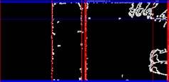
36 30 CHAPTER 4. METHODOLOGY candidates. Of course, many can already be discarded if we take into consideration various predefined values such as the minimum and maximum area of an opening. The reason why the Sobel Operator was used in addition to the Canny edge detector, is that it makes our opening detection algorithm more robust, ensuring that it does not miss any important candidates. Hough line detection on Canny edge alone was not enough to detect the proper lines for our data. Figures 4.14 and 4.15 display the results for our two data sets. Figure 4.14: Line detection for the basement data. Figure 4.15: Line detection for the seminar room data.

37 4.3. THE INTERIOR RECONSTRUCTION PIPELINE 31 In the figures above, vertical lines are drawn in red and horizontal lines are drawn in blue. We take combinations of 2 vertical and 2 horizontal lines to determine an opening candidate. There will be many redundant candidates as it can be seen in Figure 4.15, where large clusters of horizontal lines have been detected. Once we have determined all the opening candidates, we compute a vector of 14 features for each candidate as described in [4]: 1. candidate absolute area 2. candidate width / height ratio 3. candidate width / surface width ratio 4. candidate height / surface height ratio 5. distance from upper side of candidate to upper side of surface 6. distance from lower side of candidate to lower side of surface 7. distance from left side of candidate to left side of surface 8. distance from right side of candidate to right side of surface 9. root mean squared error to the best plane fitted to the rectangle surface 10. percentage of Occupied area 11. percentage of Occluded area 12. percentage of Empty area 13. number of interior rectangles 14. number of inverted U-shaped rectangles (specific to doors) In order to determine features 10, 11 and 12 we make use of the labels image. These feature vectors are used to classify the candidates. In order to train the Support Vector Machine, a small database has been put together with features of actual openings from various buildings across our campus. It is well known that a Support Vector Machine (SVM) is a learning system that performs classification tasks by constructing hyper planes in a multidimensional space. We have used a Radial Basis Function (RBF) as a kernel in a binary SVM model. After the SVM has been trained, we give each candidate as input. The SVM will tell us if the candidate represents an opening or not. In the end, we are left only with candidates that are close representatives of the ground truth we used to train the SVM with. Now that we have kept the most relevant opening candidates, many of these actually represent the same opening. We proceed by clustering the candidates by using K-Means clustering. This is a method of cluster analysis that aims to cluster n observations, our opening candidates, into k clusters in which each observation belongs to the cluster with the nearest mean. The features we use to differentiate between the candidates are the candidate s center and its absolute area, because we might have large candidates from one cluster centered at the same position with smaller candidates. After deciding which cluster the candidates belong to, we need to determine the shape of the final opening. It is important to know that the number of detected clusters is the same with the number of openings on the real surface. We proceed by choosing for each cluster the best candidate which has the largest Empty area, and the smallest Occupied and Occluded areas. This candidate is the cluster representative and is kept as the final opening that represents that particular cluster.

38 32 CHAPTER 4. METHODOLOGY Figure 4.16: Opening detection for the basement data. (a) Opening candidates (b) Clusters (c) Cluster representatives (d) Final openings Figure 4.17: From opening candidates to the final opening (basement data). As we have specified before, the basement data is very good for testing our pipeline, since for plane detection, it was very fragmented, yet the pipeline was able to accurately determine the six surfaces of the interior; for the surface labeling, it was ideal, since it contained large areas of all three labels, mainly Occluded areas, due to numerous pipes running from one side of the room to the other; for the current component, opening detection, the only opening on the surface presented in Figure 4.16 is occluded by a vertical pipe, which challenges the SVM in

39 4.3. THE INTERIOR RECONSTRUCTION PIPELINE 33 properly choosing candidates. Therefore, as it can be seen in both Figures 4.16 and 4.17, the opening candidates marked in red, are separated into three clusters. The center of each cluster has been marked with the same color as the candidates belonging to that cluster. Therefore, we are left with three possible openings, the two smaller windows that do not overlap with each other, and the larger window that overlaps with both smaller candidates. We check all the potential openings that overlap with others and always keep the one that has the largest Empty area and the smallest Occupied and Occluded area, therefore, in our example we are left with the larger candidate as final opening which corresponds to the ground truth. In the case of windows with thick frames or window mounted fans, the algorithm is able to avoid detecting multiple smaller windows, because it checks for overlapping candidates, in the end keeping the best candidate with the largest Empty area, which is always the whole window. For the seminar room data, Figures 4.18 and 4.19, the SVM s task is simplified since the openings on the surface do not present any obstructions. Almost all the opening candidates marked in red seem to overlap exactly with the real opening. Clustering is again trivial, as there are clearly two easily distinguishable clusters among the opening candidates. As before, the best candidate from each cluster is chosen as a final opening. Figure 4.18: Opening detection for the seminar room data. Notice that for the seminar room there were no overlapping clusters, therefore the final openings coincide with the computed clusters. Also, the seminar room was chosen as a second data set due to the fact that it has multiple windows on the same wall. This is just to prove that the system is able to handle multiple openings. The basement scan is important because it contains

40 34 CHAPTER 4. METHODOLOGY an occluded opening, and still, the algorithm is able to properly detect the window despite that. In the beginning we mentioned that one of the possible impediments for opening detection would be various obstructions such as occlusions, thick window frames or window mounted fans. (a) Opening candidates (b) Clusters (c) Cluster representatives (d) Final openings Figure 4.19: From opening candidates to the final opening (seminar room data). In the end, the purpose of this component is to accurately determine which regions on the surface are actual openings and which regions are actually missing information due to occlusions. After computing the final 2D openings on the depth image, we proceed to relabel all remaining Empty labels to Occluded. This yields the inpaint mask, I m, that is used for the inpainting (gap filling) algorithm [4,23]. Basically, the inpaint mask, I m, tells us what patches of the surface are actual missing information which needs to be filled in. Figures 4.16 and 4.18 show the inpaint masks for both our data sets. Notice that the amount of reconstruction required for the basement surface is significantly higher compared to the seminar room surface. The seminar room surface presents very few occlusions, whereas the basement room surface is approximately 50% occluded. In the next component we present a simple way of reconstructing the actual 3D data from the 2D depth map and the inpaint mask. Besides the inpaint mask required for the point cloud reconstruction, we also generate a simple 3D model of the interior using the detected surfaces and final 2D openings. We have also chosen the images in Figure 4.20 to show another possible opening detection for the basement data. This is one of the earlier models for the basement room, one in which the larger window would be discarded by the SVM, instead only choosing the two smaller candidates. By further increasing the SVM training database we are able to achieve the results from Figures 4.16 and 4.17.

41 4.3. THE INTERIOR RECONSTRUCTION PIPELINE 35 (a) (b) (c) (d) (e) (f) Figure 4.20: Basement room model. It is very important to mention that the scans depicted so far consist only of one scan. We present later on the results for multiple scans. Having multiple scans registered would only make the task easier, since there would be less missing information due to occlusions.

42 36 CHAPTER 4. METHODOLOGY (a) (b) (c) (d) (e) (f) (g) (h) Figure 4.21: Seminar room model.

43 4.3. THE INTERIOR RECONSTRUCTION PIPELINE Occlusion Reconstruction We are down to the last component of the pipeline. The purpose of the whole pipeline is to generate a reconstructed version of the initial point cloud, filling in the missing information induced by occlusions. This component is fairly simple, and requires the use of a gap filling algorithm [4]. Figure 4.22: The detailed Occlusion Reconstruction Pipeline. We begin by taking the original depth image, I, for every surface and apply a gap filling algorithm on it. We have used the inpainting algorithm already provided in OpenCV [3]. We use the inpaint mask computed in the previous component, I m. The result of this process is a reconstructed 2D depth image, I r, having all the missing information filled in. We then proceed to computing the mean and standard deviation of the original depth image, in the depth axis, and add Gaussian noise with the same mean and standard deviation to the newly reconstructed image, thus yielding the final reconstructed depth image of the surface, I f. The reason we add Gaussian noise to the reconstructed depth image is that the reconstructed regions have a very unnatural look and feeling. After computing the reconstructed depth image and adding noise, we then proceed by projecting I f back into 3D. This simply yields the reconstructed surface point cloud. Figures 4.24 and 4.25 depict the results on our two data sets. Light red represents the reconstructed information.

44 38 CHAPTER 4. METHODOLOGY (a) Basement depth image (b) Basement inpaint mask (c) Basement reconstructed depth image (d) Seminar room depth image (e) Seminar room inpaint mask (f) Seminar room reconstructed depth image Figure 4.23: Depth image, inpaint mask and reconstructed depth images.

45 4.3. THE INTERIOR RECONSTRUCTION PIPELINE 39 Figure 4.24: Sample reconstructed basement point cloud. Figure 4.25: Sample reconstructed seminar room point cloud.

46

47 Chapter 5 Experiments and Results 5.1 Environment All computations have been performed on an Intel Core2 Duo P8600 at 2.4GHz, 4GB of RAM, running Kubuntu LTS 64-bit. 5.2 General Results The purpose of the pipeline we presented in Figure 4.1 was to be able to run the 3DTK component on almost any computer. We reduced the point cloud to 1 point every centimeter, giving us approximately 5 million points for both our scans. The program ran smoothly without exceeding the above mentioned amount of memory. As mentioned before, we have two data sets: a scan of a basement room and a scan of the seminar room, both from the Research I building at Jacobs University Bremen. (a) Basement (b) Seminar room Figure 5.1: The two rooms used in our tests. Most of our results have already been presented in the previous sections. In this section we present the results for the other surfaces, since they have been previously omitted. Also, we present the results for not one, but four registered scans simply as a proof of concept. 41

48 42 CHAPTER 5. EXPERIMENTS AND RESULTS (a) Depth map (b) Labels (c) Enhanced edges (d) Detected lines (e) Depth mask (f) Reconstructed depth image Figure 5.2: Basement room ceiling. (a) Depth map (b) Labels (c) Enhanced edges (d) Detected lines (e) Depth mask (f) Reconstructed depth image Figure 5.3: Basement room floor.

49 5.2. GENERAL RESULTS 43 (a) Depth map (b) Labels (c) Enhanced edges (d) Detected lines (e) Depth mask (f) Reconstructed depth image Figure 5.4: Basement room wall 1. (a) Depth map (b) Labels (c) Enhanced edges (d) Detected lines (e) Depth mask (f) Reconstructed depth image Figure 5.5: Basement room wall 2. (a) Depth map (b) Labels (c) Enhanced edges (d) Detected lines (e) Depth mask (f) Reconstructed depth image Figure 5.6: Basement room wall 3.

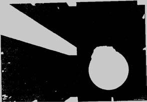
50 44 CHAPTER 5. EXPERIMENTS AND RESULTS Notice that the walls do not necessarily present any interesting features. They mostly consist of Occupied and Occluded labels since they have no openings. The anomalies are the ceiling and the roof which present a circular pattern of Empty labels. There is no opening detected here simply because if we take a look at the possible candidates, there are no rectangles that could be formed and have a high Empty area. The reason why these circular areas appear is that the scanner does not have a perfect 180 view, therefore when it spins, it leaves such patterns right above and below. Of course, the size of these circular patterns depend on the scanner. One way of circumventing this is by detecting such circular patterns above and below the origin of the scan and flooding the Empty labels with Occluded ones, since that area is missing information. From a raytracing point of view, we simply consider that the scanner is able to see in all directions, that is why these areas are attributed the wrong label. A better way of removing such anomalies is by acquiring multiple scans and registering them using the slam6d component of 3DTK. We now present the labeling results (Figure 5.7) for 4 registered scans taken in the basement room. Acquiring multiple scans does not only allow us to eliminate anomalies, it also enables us to significantly reduce the Occluded area. All 4 registered scans and room model are presented in Figure 5.8. As mentioned before, the size of the database used to train the Support Vector Machine greatly influences the outcome of the opening detection component. Figures 5.9 and 5.10 depict multiple results for opening detection. Notice that in the basement data there are some differences from one result to the other. When clustering, multiple clusters are detected in some of the results, nevertheless the opening is correctly detected in the end. Looking at the final openings, we notice that not always the larger window gets chosen as final. This is a matter of perspective, if we consider the pipe blocking the view to the opening as part of the wall, then yes, the two smaller windows detected would be appropriate, otherwise, the larger window should be chosen. This can easily be controlled by adjusting various parameters, such as the allowed Occupied and Occluded areas of the openings, or by simply carefully choosing the training data for the SVM. For the seminar room data, Figure 5.10, there is not much variance. Final openings always get chosen correctly, and the clusters never show much variance. There is always one cluster per opening, since there is not much ambiguity in the scene at hand. The purpose of window detection is merely to decide upon what Empty labels truly represent empty space. This is required to generate the inpaint mask required for the 3D reconstruction. The results for the 3D reconstruction for our data sets have already been presented in Figures 4.24 and 4.25.

51 5.2. GENERAL RESULTS 45 (a) Window wall (1 scan) (b) Window wall (4 scans) (c) Ceiling (1 scan) (d) Ceiling (4 scans) (e) Floor (1 scan) (f) Floor (4 scans) (g) Wall (1 scan) (h) Wall (4 scans) (i) Wall (1 scan) (j) Wall (4 scans) (k) Wall (1 scan) (l) Wall (4 scans) Figure 5.7: Basement room labeling comparison between 1 scan and 4 registered scans.

52 46 CHAPTER 5. EXPERIMENTS AND RESULTS Figure 5.8: Basement room - all 4 registered scans and model (multiple views).

53 5.2. GENERAL RESULTS 47 Figure 5.9: Various results for opening detection (detected clusters and final openings).

54 48 CHAPTER 5. EXPERIMENTS AND RESULTS Figure 5.10: Various results for opening detection (detected clusters and final openings).