Gene Finding & Review

Transcription

1 Gene Finding & Review Michael Schatz Bioinformatics Lecture 4 Quantitative Biology 2010

2 Illumina DNA Sequencing Pacific Biosciences

3 Outline 1. 'Semantic' Sequence Analysis 1. Prokaryotic Gene Finding 2. Eukaryotic Gene Finding 3. Phylogenetic Trees (Supplemental) 2. Review 1. Exact Matching 2. Sequence Alignment 3. Genome Assembly 4. Gene Finding

4 aatgcatgcggctatgctaatgcatgcggctatgctaagctgggatccgatgacaatgcatgcggctatgctaa tgcatgcggctatgcaagctgggatccgatgactatgctaagctgggatccgatgacaatgcatgcggctatgc taatgaatggtcttgggatttaccttggaatgctaagctgggatccgatgacaatgcatgcggctatgctaatga atggtcttgggatttaccttggaatatgctaatgcatgcggctatgctaagctgggatccgatgacaatgcatgc ggctatgctaatgcatgcggctatgcaagctgggatccgatgactatgctaagctgcggctatgctaatgcatg cggctatgctaagctgggatccgatgacaatgcatgcggctatgctaatgcatgcggctatgcaagctgggatc ctgcggctatgctaatgaatggtcttgggatttaccttggaatgctaagctgggatccgatgacaatgcatgcgg ctatgctaatgaatggtcttgggatttaccttggaatatgctaatgcatgcggctatgctaagctgggaatgcatg cggctatgctaagctgggatccgatgacaatgcatgcggctatgctaatgcatgcggctatgcaagctgggatc cgatgactatgctaagctgcggctatgctaatgcatgcggctatgctaagctcatgcggctatgctaagctggg aatgcatgcggctatgctaagctgggatccgatgacaatgcatgcggctatgctaatgcatgcggctatgcaag ctgggatccgatgactatgctaagctgcggctatgctaatgcatgcggctatgctaagctcggctatgctaatga atggtcttgggatttaccttggaatgctaagctgggatccgatgacaatgcatgcggctatgctaatgaatggtc ttgggatttaccttggaatatgctaatgcatgcggctatgctaagctgggaatgcatgcggctatgctaagctgg gatccgatgacaatgcatgcggctatgctaatgcatgcggctatgcaagctgggatccgatgactatgctaagc tgcggctatgctaatgcatgcggctatgctaagctcatgcgg

5 aatgcatgcggctatgctaatgcatgcggctatgctaagctgggatccgatgacaatgcatgcggctatgctaa tgcatgcggctatgcaagctgggatccgatgactatgctaagctgggatccgatgacaatgcatgcggctatgc taatgaatggtcttgggatttaccttggaatgctaagctgggatccgatgacaatgcatgcggctatgctaatga atggtcttgggatttaccttggaatatgctaatgcatgcggctatgctaagctgggatccgatgacaatgcatgc ggctatgctaatgcatgcggctatgcaagctgggatccgatgactatgctaagctgcggctatgctaatgcatg cggctatgctaagctgggatccgatgacaatgcatgcggctatgctaatgcatgcggctatgcaagctgggatc ctgcggctatgctaatgaatggtcttgggatttaccttggaatgctaagctgggatccgatgacaatgcatgcgg ctatgctaatgaatggtcttgggatttaccttggaatatgctaatgcatgcggctatgctaagctgggaatgcatg Gene! cggctatgctaagctgggatccgatgacaatgcatgcggctatgctaatgcatgcggctatgcaagctgggatc cgatgactatgctaagctgcggctatgctaatgcatgcggctatgctaagctcatgcggctatgctaagctggg aatgcatgcggctatgctaagctgggatccgatgacaatgcatgcggctatgctaatgcatgcggctatgcaag ctgggatccgatgactatgctaagctgcggctatgctaatgcatgcggctatgctaagctcggctatgctaatga atggtcttgggatttaccttggaatgctaagctgggatccgatgacaatgcatgcggctatgctaatgaatggtc ttgggatttaccttggaatatgctaatgcatgcggctatgctaagctgggaatgcatgcggctatgctaagctgg gatccgatgacaatgcatgcggctatgctaatgcatgcggctatgcaagctgggatccgatgactatgctaagc tgcggctatgctaatgcatgcggctatgctaagctcatgcgg

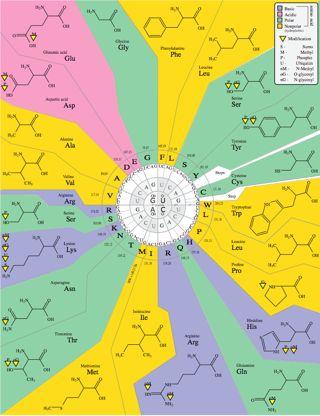
6 Genes to Proteins

7 Bacterial Gene Finding and Glimmer (also Archaeal and viral gene finding) Arthur L. Delcher and Steven Salzberg Center for Bioinformatics and Computational Biology University of Maryland

8 Outline A (very) brief overview of microbial gene-finding Glimmer1 & 2 Interpolated Markov Model (IMM) Interpolated Context Model (ICM) Glimmer3 Reducing false positives Improving coding initiation site predictions Running Glimmer3

9 Step One Find open reading frames (ORFs). TAGAAAAATGGCTCTTTAGATAAATTTCATGAAAAATATTGA Stop codon Stop codon

10 Step One Find open reading frames (ORFs). Stop codon Reverse strand ATCTTTTTACCGAGAAATCTATTTAAAGTACTTTTTATAACT TAGAAAAATGGCTCTTTAGATAAATTTCATGAAAAATATTGA Stop codon Shifted Stop Stop codon But ORFs generally overlap

11 Campylobacter jejuni RM %GC All ORFs on both strands shown - color indicates reading frame Longest ORFs likely to be protein-coding genes Note the low GC content All genes are ORFs but not all ORFs are genes

12 Campylobacter jejuni RM %GC Campylobacter jejuni RM %GC

13 Mycobacterium smegmatis MC2 67.4%GC Note what happens in a high-gc genome

14 Mycobacterium smegmatis MC2 67.4%GC Mycobacterium smegmatis MC2 67.4%GC

15 The Problem Need to decide which orfs are genes. Then figure out the coding start sites Can do homology searches but that won t find novel genes Besides, there are errors in the databases Generally can assume that there are some known genes to use as training set. Or just find the obvious ones

16 Probabilistic Methods Create models that have a probability of generating any given sequence. Train the models using examples of the types of sequences to generate. The score of an orf is the probability of the model generating it. Can also use a negative model (i.e., a model of nonorfs) and make the score be the ratio of the probabilities (i.e., the odds) of the two models. Use logs to avoid underflow

17 Fixed-Order Markov Models k th -order Markov model bases the probability of an event on the preceding k events. Example: With a 3 rd -order model the probability of this sequence: would be: Target!Context " CTAG AT" " P(G CTA)! P(A TAG)! P(T AGA) " Target! Context

18 Fixed-Order Markov Models Advantages: Easy to train. Count frequencies of (k+1)-mers in training data. Easy to compute probability of sequence. Disadvantages: Many (k+1)-mers may be undersampled in training data. Models data as fixed-length chunks. Fixed-Length Context Target ACGT AGTTCAGTA

19 Interpolated Markov Models (IMM) Introduced in Glimmer 1.0 Salzberg, Delcher, Kasif & White, NAR 26, Probability of the target position depends on a variable number of previous positions (sometimes 2 bases, sometimes 3, 4, etc.) How many is determined by the specific context. E.g., for context ggtta the next position might depend on previous 3 bases tta. But for context catta all 5 bases might be used.

20 IMMs vs Fixed-Order Models Performance IMM generally should do at least as well as a fixedorder model. Some risk of overtraining. IMM result can be stored and used like a fixedorder model. IMM will be somewhat slower to train and will use more memory. Variable-Length Context Target ACGT AGTTCAGTA

21 Interpolated Context Model (ICM) Introduced in Glimmer 2.0 Delcher, Harmon, et al., Nucl. Acids Res. 27, Doesn t require adjacent bases in the window preceding the target position. Choose set of positions that are most informative about the target position. Variable-Position Context Target ACGTAGTTCAGTA

22 ICM For all windows compare distribution at each context position with target position ************* Choose position with max mutual information p( x, y) I( X ; Y ) =!! p( x, y)log p ( x ) p ( y ) x y Compare

23 ICM Continue for windows with fixed base at chosen positions **** A ******** Compare Recurse until too few training windows Result is a tree depth is # of context positions used Then same interpolation as IMM, between node and parent in tree

24 Overlapping Orfs Glimmer1 & 2 used rules. For overlapping orfs A and B, the overlap region AB is scored separately: If AB scores higher in A s reading frame, and A is longer than B, then reject B. If AB scores higher in B s reading frame, and B is longer than A, then reject A. Otherwise, output both A and B with a suspicious tag. Also try to move start site to eliminate overlaps. Leads to high false-positive rate, especially in high-gc genomes.

25 Glimmer3 Uses a dynamic programming algorithm to choose the highest-scoring set of orfs and start sites. Not quite an HMM Allows small overlaps between genes small is user-defined Scores of genes are not necessarily probabilities. Score includes component for likelihood of start site

26 Reverse Scoring In Glimmer3 orfs are scored from 3 end to 5 end, i.e., from stop codon back toward start codon. Helps find the start site. The start should appear near the peak of the cumulative score in this direction. Keeps the context part of the model entirely in the coding portion of gene, which it was trained on.

27 Reverse Scoring

28

29 CBB 231 / COMPSCI 261 W.H. Majoros

30 Exons, Introns, and Genes Exon Gene Intron Exon The human genome: 23 pairs of chromosomes 2.9 billion A s, T s, C s, G s ~22,000 genes (?) ~1.4% of genome is coding

31 Eukaryotic Gene Syntax ATG complete mrna coding segment TGA exon intron exon intron exon ATG... GT AG... GT AG... TGA start codon donor site acceptor site donor site acceptor site stop codon Regions of the gene outside of the CDS are called UTR s (untranslated regions), and are mostly ignored by gene finders, though they are important for regulatory functions.

32 Types of Exons Three types of exons are defined, for convenience: initial exons extend from a start codon to the first donor site; internal exons extend from one acceptor site to the next donor site; final exons extend from the last acceptor site to the stop codon; single exons (which occur only in intronless genes) extend from the start codon to the stop codon:

33 Representing Gene Syntax with ORF Graphs After identifying the most promising (i.e., highest-scoring) signals in an input sequence, we can apply the gene syntax rules to connect these into an ORF graph: An ORF graph represents all possible gene parses (and their scores) for a given set of putative signals. A path through the graph represents a single gene parse.

34 Conceptual Gene-finding Framework TATTCCGATCGATCGATCTCTCTAGCGTCTACG CTATCATCGCTCTCTATTATCGCGCGATCGTCG ATCGCGCGAGAGTATGCTACGTCGATCGAATTG identify most promising signals, score signals and content regions between them; induce an ORF graph on the signals find highest-scoring path through ORF graph; interpret path as a gene parse = gene structure

35 The Notion of an Optimal Gene Structure If we could enumerate all putative gene structures along the x-axis and graph their scores according to some function f(x), then the highest-scoring parse would be denoted argmax f(x), and its score would be denoted max f(x). A gene finder will often find the local maximum rather than the global maximum.

36 Hidden Markov Models (HMMs) Steven Salzberg CMSC 828N, Univ. of Maryland

37 What is an HMM? Dynamic Bayesian Network A set of states {Fair, Biased} for coin tossing {Gene, Not Gene} for Bacterial Gene {Intergenic, Exon, Intron} for Eukaryotic Gene A set of emission characters E={H,T} for coin tossing E={1,2,3,4,5,6} for dice tossing E={A,C,G,T} = for DNA State-specific emission probabilities P(H Fair) =.5, P(T Fair) =.5, P(H Biased) =.9, P(T Biased) =.1 P(A Gene) =.9, P(A Not Gene) =.1 A probability of taking a transition P(s i =Fair s i-1 =Fair) =.9, P(s i =Bias s i-1 = Fair).1 P(s i =Exon s i-1 =Intergenic),

38 Why Hidden? Observers can see the emitted symbols of an HMM but have no ability to know which state the HMM is currently in. But we can infer the most likely hidden states of an HMM based on the given sequence of emitted symbols. HTHHTTHHHTHTHTHHTHHHHHHTHTHH!

39 HMM Example - Casino Coin Fair 0.8 Unfair State transition probs. States Symbol emission probs. H T H T HTHHTTHHHTHTHTHHTHHHHHHTHTHH! FFFFFFUUUFFFFFFUUUUUUUFFFFFF! Observation Symbols Observation Sequence State Sequence Motivation: Given a sequence of H & Ts, can you tell at what times the casino cheated? Slide credit: Fatih Gelgi, Arizona State U.

40 Three classic HMM problems 1. Evaluation: given a model and an output sequence, what is the probability that the model generated that output? To answer this, we consider all possible paths through the model Example: we might have a set of HMMs representing protein families -> pick the model with the best score

41 Three classic HMM problems 2. Decoding: given a model and an output sequence, what is the most likely state sequence through the model that generated the output? A solution to this problem gives us a way to match up an observed sequence and the states in the model. AAAGC ATG CAT TTA ACG AGA GCA CAA GGG CTC TAA TGCCG The sequence of states is an annotation of the generated string each nucleotide is generated in intergenic, start/stop, coding state

42 Three classic HMM problems 3. Learning: given a model and a set of observed sequences, how do we set the model s parameters so that it has a high probability of generating those sequences? This is perhaps the most important, and most difficult problem. A solution to this problem allows us to determine all the probabilities in an HMMs by using an ensemble of training data

43 Solving the Evaluation problem: The Forward algorithm To solve the Evaluation problem (probability that the model generated the sequence), we use the HMM and the data to build a trellis Filling in the trellis will give tell us the probability that the HMM generated the data by finding all possible paths that could do it

44 Our sample HMM Let S 1 be initial state, S 2 be final state

45 A trellis for the Forward Algorithm S 1 Time t=0 t=1 t=2 t=3 1.0 (0.6)(0.8)(1.0) State S (0.9)(0.3)(0) A C C Output:

46 A trellis for the Forward Algorithm S 1 Time t=0 t=1 t=2 t=3 1.0 (0.6)(0.8)(1.0) (0.6)(0.2)(0.48) = State S (0.9)(0.3)(0) (0.9)(0.7)(0.2) =.222 A C C Output:

47 A trellis for the Forward Algorithm S 1 Time t=0 t=1 t=2 t=3 1.0 (0.6)(0.8)(1.0) (0.6)(0.2)(0.48) (0.6)(0.2)(.0756) = State S (0.9)(0.3)(0) (0.9)(0.7)(0.2) = (0.9)(0.7)(0.222) A C C Output:

48 Probability of the model The Forward algorithm computes P(y M) If we are comparing two or more models, we want the likelihood that each model generated the data: P(M y) Use Bayes law: P(M y) = P(y M)P(M) P(y) Since P(y) is constant for a given input, we just need to maximize P(y M)P(M)

49 Solving the Decoding Problem: The Viterbi algorithm To solve the decoding problem (find the most likely sequence of states), we evaluate the Viterbi algorithm V i ( t) = % 0 : t = 0"i # S ' I & 1 : t = 0"i = S I ' ( max V j (t $1)a ji b ji (y) : t > 0 Where V i (t) is the probability that the HMM is in state i after generating the sequence y 1,y 2,,y t, following the most probable path in the HMM

50 A trellis for the Viterbi Algorithm Time S 1 t=0 t=1 t=2 t=3 1.0 (0.6)(0.8)(1.0) max 0.48 State S max (0.9)(0.3)(0) 0.20 A C C Output:

51 A trellis for the Viterbi Algorithm Time S 1 t=0 t=1 t=2 t=3 1.0 (0.6)(0.8)(1.0) max 0.48 (0.6)(0.2)(0.48) max max(.0576,.018) =.0576 State S max (0.9)(0.3)(0) 0.20 max (0.9)(0.7)(0.2) max(.126,.096) =.126 A C C Output:

52 A trellis for the Viterbi Algorithm S 1 Time t=0 t=1 t=2 t=3 1.0 (0.6)(0.8)(1.0) max 0.48 (0.6)(0.2)(0.48) (0.6)(0.2)(0.0576) max( ,.01134).0576 = max max State S max (0.9)(0.3)(0) 0.20 max (0.9)(0.7)(0.2) max max(.01152,.07938).126 = (0.9)(0.7)(0.126) A C C Output:

53 A trellis for the Viterbi Algorithm Time S 1 t=0 t=1 t=2 t=3 1.0 (0.6)(0.8)(1.0) max 0.48 (0.6)(0.2)(0.48) max.0576 (0.6)(0.2)(0.0576) max State S max (0.9)(0.3)(0) 0.20 max (0.9)(0.7)(0.2).126 max (0.9)(0.7)(0.126) A C C Output: S Parse: 1 S 2 S 2

54 Learning in HMMs: The E-M algorithm In order to learn the parameters in an empty HMM, we need: The topology of the HMM Data - the more the better The learning algorithm is called Expectation- Maximization or E-M Also called the Forward-Backward algorithm Also called the Baum-Welch algorithm See Supplemental Slides

55 Eukaryotic Gene Finding with GlimmerHMM Mihaela Pertea Assistant Research Scientist CBCB

56 HMMs and Gene Structure Nucleotides {A,C,G,T} are the observables Different states generate nucleotides at different frequencies A simple HMM for unspliced genes: A T G T A A AAAGC ATG CAT TTA ACG AGA GCA CAA GGG CTC TAA TGCCG The sequence of states is an annotation of the generated string each nucleotide is generated in intergenic, start/stop, coding state

57 HMMs & Geometric Feature Lengths geometric distribution exon length

58 Generalized HMMs Summary GHMMs generalize HMMs by allowing each state to emit a subsequence rather than just a single symbol Whereas HMMs model all feature lengths using a geometric distribution, coding features can be modeled using an arbitrary length distribution in a GHMM Emission models within a GHMM can be any arbitrary probabilistic model ( submodel abstraction ), such as a neural network or decision tree GHMMs tend to have many fewer states => simplicity & modularity

59 GlimmerHMM architecture Four exon types Exon0 Exon1 Exon2 I0 I1 I2 Phase-specific introns Init Exon Exon Sngl Term Exon + forward strand - backward strand Term Exon I0 Exon0 Intergenic Exon Sngl I1 Exon1 Init Exon I2 Exon2 Uses GHMM to model gene structure (explicit length modeling) WAM and MDD for splice sites ICMs for exons, introns and intergenic regions Different model parameters for regions with different GC content Can emit a graph of highscoring ORFS

60 Signal Sensors Signals short sequence patterns in the genomic DNA that are recognized by the cellular machinery.

61 Identifying Signals In DNA We slide a fixed-length model or window along the DNA and evaluate score (signal) at each point: Signal sensor ACTGATGCGCGATTAGAGTCATGGCGATGCATCTAGCTAGCTATATCGCGTAGCTAGCTAGCTGATCTACTATCGTAGC When the score is greater than some threshold (determined empirically to result in a desired sensitivity), we remember this position as being the potential site of a signal. The most common signal sensor is the Weight Matrix: A = 31% T = 28% C = 21% G = 20% A = 18% T = 32% C = 24% G = 26% A 100% T 100% G 100% A = 19% T = 20% C = 29% G = 32% A = 24% T = 18% C = 26% G = 32%

62 Splice site prediction 16bp 24bp The splice site score is a combination of: first or second order inhomogeneous Markov models on windows around the acceptor and donor sites MDD decision trees longer Markov models to capture difference between coding and noncoding on opposite sides of site (optional) maximal splice site score within 60 bp (optional)

63 Coding vs Non-coding A three-periodic ICM uses three ICMs in succession to evaluate the different codon positions, which have different statistics: P[C M 0 ] P[G M1 ] P[A M2 ] ICM 0 ICM 1 ICM 2 ATC GAT CGA TCA GCT TAT CGC ATC The three ICMs correspond to the three phases. Every base is evaluated in every phase, and the score for a given stretch of (putative) coding DNA is obtained by multiplying the phase-specific probabilities in a mod 3 fashion: GlimmerHMM uses 3-periodic ICMs for coding and homogeneous (non-periodic) ICMs for noncoding DNA.

64 GlimmerHMM architecture Four exon types Exon0 Exon1 Exon2 I0 I1 I2 Phase-specific introns Init Exon Exon Sngl Term Exon + forward strand - backward strand Term Exon I0 Exon0 Intergenic Exon Sngl I1 Exon1 Init Exon I2 Exon2 Uses GHMM to model gene structure (explicit length modeling) WAM and MDD for splice sites ICMs for exons, introns and intergenic regions Different model parameters for regions with different GC content Can emit a graph of highscoring ORFS

65 Gene Prediction with a GHMM Given a sequence S, we would like to determine the parse! of that sequence which segments the DNA into the most likely exon/intron structure: prediction parse! sequence S initial interior final AGCTAGCAGTCGATCATGGCATTATCGGCCGTAGTACGTAGCAGTAGCTAGTAGCAGTCGATAGTAGCATTATCGGCCGTAGCTACGTAGCGTAGCTC The parse! consists of the coordinates of the predicted exons, and corresponds to the precise sequence of states during the operation of the GHMM (and their duration, which equals the number of symbols each state emits). This is the same as in an HMM except that in the HMM each state emits bases with fixed probability, whereas in the GHMM each state emits an entire feature such as an exon or intron.

66 Evaluation of Gene Finding Programs Nucleotide level accuracy TN FN TP FP TN FN TP FN TN REALITY PREDICTION Sensitivity: Specificity:

67 More Measures of Prediction Accuracy Exon level accuracy REALITY WRONG EXON CORRECT EXON MISSING EXON PREDICTION

68 GlimmerHMM on human data Nuc Nuc Nuc Exon Exon Exon Exact Sens Spec Acc Sens Spec Acc Genes GlimmerHMM 86% 72% 79% 72% 62% 67% 17% Genscan 86% 68% 77% 69% 60% 65% 13% GlimmerHMM s performace compared to Genscan on 963 human RefSeq genes selected randomly from all 24 chromosomes, non-overlapping with the training set. The test set contains 1000 bp of untranslated sequence on either side (5' or 3') of the coding portion of each gene.

69 GlimmerHMM is a high-performance ab initio gene finder Arabidopsis thaliana test results Nucleotide Exon Gene Sn Sp Acc Sn Sp Acc Sn Sp Acc GlimmerHMM SNAP Genscan All three programs were tested on a test data set of 809 genes, which did not overlap with the training data set of GlimmerHMM. All genes were confirmed by full-length Arabidopsis cdnas and carefully inspected to remove homologues.

70 Summary Prokaryotic gene finding distinguishes between genes and random ORFs Prokaryotic genes have simple structure and are largely homogenous, making it relatively easy to recognize their sequence composition Eukaryotic gene finding identifies the genome-wide most probable gene models (set of exons) GHMM to enforce overall gene structure, separate models to score splicing/transcription signals Accuracy depends to a large extent on the quality of the training data All future genome projects will be accompanied by mrnaseq

71 Break

72 Review

73 Exact Matching Explain the Brute Force search algorithm (algorithm sketch, running time, space requirement) 1. Suffix Arrays 2. Suffix Trees 3. Hash Tables 4. How many times do we expected GATTACA or GATTACA*2 or GATTACA*3 to be in the genome?

74 Sequence Alignment 1. What is a good scoring scheme for aligning: English words? Illumina Reads? Gene Sequences? Genomes? 2. Explain Dynamic Programming for Sequence Alignment 3. BLAST 4. MUMmer 5. Bowtie

75 Graphs and Assembly 1. How do I compute the shortest path between 2 nodes and how long does it take? 2. Mark connected components in a graph? 3. Shortest path visiting all nodes? 4. Describe Genome Assembly 5. How do we detect mis-assemblies?

76 Gene Finding 1. Describe Prokaryotic Gene Finding 2. Describe Eukaryotic gene finding 3. What is an Markov Chain? IMM? ICM? HMM? GHMM? 4. What do the Forward and Viterbi Algorithms Compute

77 1. Order these running times CS Fundamentals O(lg n), O(2 n ), O(n 100 ), O(n 2 ), O(n!) O(nlgn), O(n(lgn)(lgn)), O(1), O(1.5 n ) 2. Describe Selection Sort 3. QuickSort 4. Bucket Sort 5. Describe Recursion 6. Dynamic Programming 7. Branch-and-Bound 8. Greedy Algorithm 9. Describe an NP-complete problem

78 Supplemental

79

80 Learning in HMMs: The E-M algorithm In order to learn the parameters in an empty HMM, we need: The topology of the HMM Data - the more the better The learning algorithm is called Estimate- Maximize or E-M Also called the Forward-Backward algorithm Also called the Baum-Welch algorithm 80

81 An untrained HMM 81

82 Some HMM training data CACAACAAAACCCCCCACAA ACAACACACACACACACCAAAC CAACACACAAACCCC CAACCACCACACACACACCCCA CCCAAAACCCCAAAAACCC ACACAAAAAACCCAACACACAACA ACACAACCCCAAAACCACCAAAAA 82

83 Step 1: Guess all the probabilities We can start with random probabilities, the learning algorithm will adjust them If we can make good guesses, the results will generally be better 83

84 Step 2: the Forward algorithm Reminder: each box in the trellis contains a value! i (t)! i (t) is the probability that our HMM has generated the sequence y 1, y 2,, y t and has ended up in state i. 84

85 Reminder: notations sequence of length T: all sequences of length T: Path of length T+1 generates Y: All paths: X 1 T +1 y 1 T Y 1 T x 1 T +1 85

86 Step 3: the Backward algorithm Next we need to compute " i (t) using a Backward computation " i (t) is the probability that our HMM will generate the rest of the sequence y t+1,y t+2,, y T beginning in state i 86

87 A trellis for the Backward Algorithm S 1 Time t=0 t=1 t=2 t= (0.6)(0.2)(0.0) 0.0 State S (0.9)(0.7)(1.0) 1.0 A C C Output: 87

88 A trellis for the Backward Algorithm (2) S 1 Time t=0 t=1 t=2 t= (0.6)(0.2)(0.2) =.15 (0.6)(0.2)(0.0) State S = (0.9)(0.7)(0.63) (0.9)(0.7)(1.0) A C C Output: 88

89 A trellis for the Backward Algorithm (3) S 1 Time t=0 t=1 t=2 t= (0.6)(0.8)(0.15) = (0.6)(0.2)(0.2) (0.6)(0.2)(0.0) State S = (0.9)(0.3)(0.415) (0.9)(0.7)(0.63) (0.9)(0.7)(1.0) A C C Output: 89

90 Step 4: Re-estimate the probabilities After running the Forward and Backward algorithms once, we can re-estimate all the probabilities in the HMM # SF is the prob. that the HMM generated the entire sequence Nice property of E-M: the value of # SF never decreases; it converges to a local maximum We can read off # and " values from Forward and Backward trellises 90

91 Compute new transition probabilities $ is the probability of making transition i-j at time t, given the observed output $ is dependent on data, plus it only applies for one time step; otherwise it is just like a ij (t) " ij t ( ) = P(X t = i, X t +1 = j y 1 T ) " ij t ( ) = # i(t $1)a ij b ij (y t )% j (t) # SF 91

92 What is gamma? Sum $ over all time steps, then we get the expected number of times that the transition i-j was made while generating the sequence Y: C 1 = T # t=1 " ij (t) 92

93 How many times did we leave i? Sum $ over all time steps and all states that can follow i, then we get the expected number of times that the transition i-x as made for any state x: C 2 = T ## " ik (t) t=1 k 93

94 Recompute transition probability a ij = C 1 C 2 In other words, probability of going from state i to j is estimated by counting how often we took it for our data (C1), and dividing that by how often we went from i to other states (C2) 94

95 Recompute output probabilities Originally these were b ij (k) values We need: expected number of times that we made the transition i-j and emitted the symbol k The expected number of times that we made the transition i-j 95

96 New estimate of b ij (k) # " ij (t) b ij (k) = t:y t = k T # " ij (t) t=1 96

97 Step 5: Go to step 2 Step 2 is Forward Algorithm Repeat entire process until the probabilities converge Usually this is rapid, iterations Estimate-Maximize because the algorithm first estimates probabilities, then maximizes them based on the data Forward-Backward refers to the two computationally intensive steps in the algorithm 97

98 Multiple Alignment & Phylogenetic Trees bioalgorithms.info

99 Rooted and Unrooted Trees Carp Trout root: common ancestor Zebrafish Salmon Human Mouse Chicken Salmon Unrooted trees give no information about the order of events 99

100 Unrooted vs. Rooted Trees An unrooted tree gives information about the relationships between taxa. (2k 5)!/2 k 3 (k 3)! trees with k leaves A rooted gene tree gives information about the order of events. (2k 3)!/2 k 2 (k 2)! trees with k leaves 100

101 Multiple Alignment versus Pairwise Alignment Up until now we have only tried to align two sequences.!

102 Multiple Alignment versus Pairwise Alignment Up until now we have only tried to align two sequences.! What about more than two? And what for?!

103 Multiple Alignment versus Pairwise Alignment Up until now we have only tried to align two sequences.! What about more than two? And what for?! A faint similarity between two sequences becomes significant if present in many! Multiple alignments can reveal subtle similarities that pairwise alignments do not reveal!

104 Generalizing the Notion of Pairwise Alignment Alignment of 2 sequences is represented as a 2-row matrix In a similar way, we represent alignment of 3 sequences as a 3-row matrix A T _ G C G _ A _ C G T _ A A T C A C _ A Score: more conserved columns, better alignment

105 2-D vs 3-D Alignment Grid V W 2-D edit graph 3-D edit graph

106 Multiple Alignment: Dynamic Programming s i,j,k = max s i-1,j-1,k-1 + "(v i, w j, u k )! s i-1,j-1,k! + " (v i, w j, _ )! s i-1,j,k-1! + " (v i, _, u k )! s i,j-1,k-1! + " (_, w j, u k )! s i-1,j,k! + " (v i, _, _)! s i,j-1,k! + " (_, w j, _)! s i,j,k-1! + " (_, _, u k )! cube diagonal: no indels face diagonal: one indel edge diagonal: two indels "(x, y, z) is an entry in the 3-D scoring matrix

107 Multiple Alignment: Running Time For 3 sequences of length n, the run time is 7n 3 ; O(n 3 ) For k sequences, build a k-dimensional Manhattan, with run time (2 k -1)(n k ); O(2 k n k ) Conclusion: dynamic programming approach for alignment between two sequences is easily extended to k sequences but it is impractical due to exponential running time Apply heuristics to efficiently compute approx. solutions

108 ClustalW Popular multiple alignment tool today W stands for weighted (different parts of alignment are weighted differently). Three-step process 1.) Construct pairwise alignments 2.) Build Guide Tree 3.) Progressive Alignment guided by the tree

109 Step 1: Pairwise Alignment Aligns each sequence again each other giving a similarity matrix Similarity = exact matches / sequence length (percent identity) v 1 v 2 v 3 v 4 v 1 - v v v (.17 means 17 % identical)

110 Step 2: Guide Tree Create Guide Tree using the similarity matrix ClustalW uses the neighbor-joining method Iteratively merge the pair that are close to one another, but far from others Guide tree roughly reflects evolutionary relations

111 Step 2: Guide Tree (cont d) v 1 v 2 v 3 v 4 v 1 - v v v v 1 v 3 v 4 v 2 Calculate: v 1,3 = alignment (v 1, v 3 ) v 1,3,4 = alignment((v 1,3 ),v 4 ) v 1,2,3,4 = alignment((v 1,3,4 ),v 2 )

112 Step 3: Progressive Alignment Start by aligning the two most similar sequences Following the guide tree, add in the next sequences, aligning to the existing alignment Insert gaps as necessary FOS_RAT FOS_MOUSE FOS_CHICK FOSB_MOUSE FOSB_HUMAN PEEMSVTS-LDLTGGLPEATTPESEEAFTLPLLNDPEPK-PSLEPVKNISNMELKAEPFD PEEMSVAS-LDLTGGLPEASTPESEEAFTLPLLNDPEPK-PSLEPVKSISNVELKAEPFD SEELAAATALDLG----APSPAAAEEAFALPLMTEAPPAVPPKEPSG--SGLELKAEPFD PGPGPLAEVRDLPG-----STSAKEDGFGWLLPPPPPPP LPFQ PGPGPLAEVRDLPG-----SAPAKEDGFSWLLPPPPPPP LPFQ.. : **. :.. *:.* *. * **: Dots and stars show how well-conserved a column is.