Rasterization. Computer Graphics Fabio Pellacini and Steve Marschner

Transcription

1 Rasterization 1

2 Approaches to rendering Rasterization: project each object onto image real-time rendering and GPUs foreach object in scene: foreach pixel in image: if object affects pixel: do_something() Raytracing: project each pixel onto the objects offline rendering, realistic rendering foreach pixel in image: foreach object in scene: if object affects pixel: do_something() 2

3 The graphics pipeline The standard approach to object-order graphics Implemented in hardware, e.g. graphics cards in PCs amazing performance: millions of triangles per frame We ll focus on an abstract version of hardware pipeline Pipeline because of the many stages Very parallelizable, leading to remarkable performance of graphics cards (many times the flops of CPUs at ~1/5 clock speed) Minimal support for shapes: points, lines, triangles other shapes need to be translated into the above ones Trend over the decades: toward minimal primitives simple, uniform, repetitive: good for parallelism 3

4 Pipeline VERTS. INDICES TRANSFORMED VERTICES ASSEMBLED PRIMITIVES PIXEL FRAGMENTS SHADED FRAGMENTS FINAL IMAGE VERTEX PROCESSING PRIMITIVE ASSEMBLY RASTERIZATION FRAGMENT PROCESSING FRAMEBUFFER PROCESSING Transform vertices and projection Assemble vertices into primitives Fragment generation Lighting z-buffer Compositing 4

5 Programmable Pipeline VERTS. INDICES TRANSFORMED VERTICES ASSEMBLED PRIMITIVES PIXEL FRAGMENTS SHADED FRAGMENTS FINAL IMAGE VERTEX PROCESSING PRIMITIVE ASSEMBLY RASTERIZATION FRAGMENT PROCESSING FRAMEBUFFER PROCESSING VERTEX SHADER n l+r r l 0 l r 0 2n b+t 0 t b b t 0 f+n 2fn n f f n CONSTANTS TEXTURES FRAGMENT SHADER

6 Projection 6

7 Pipeline VERTS. INDICES TRANSFORMED VERTICES ASSEMBLED PRIMITIVES PIXEL FRAGMENTS SHADED FRAGMENTS FINAL IMAGE VERTEX PROCESSING PRIMITIVE ASSEMBLY RASTERIZATION FRAGMENT PROCESSING FRAMEBUFFER PROCESSING Transform vertices and projection Assemble vertices into primitives Fragment generation Lighting z-buffer Compositing 7

8 Parallel projection To render an image of a 3D scene, we project it onto a plane Simplest kind of projection is parallel projection image projection plane scene 8

9 Orthographic projection projection plane parallel to a coordinate plane projection direction perpendicular to projection plane [Carlbom & Paciorek 78] 9

10 Off-axis parallel projection [Carlbom & Paciorek 78] axonometric: projection plane perpendicular to projection direction but not parallel to coordinate planes oblique: projection plane parallel to a coordinate plane but not perpendicular to projection direction. 10

11 Orthographic projection In graphics usually we lump axonometric with orthographic Projection plane perpendicular to projection direction Image height determines size of objects in image 11

12 Orthographic projection In graphics usually we lump axonometric with orthographic Projection plane perpendicular to projection direction Image height determines size of objects in image 11

13 Orthographic projection In graphics usually we lump axonometric with orthographic Projection plane perpendicular to projection direction Image height determines size of objects in image 11

14 Orthographic projection In graphics usually we lump axonometric with orthographic Projection plane perpendicular to projection direction Image height determines size of objects in image 11

15 Oblique projection View direction no longer coincides with projection plane normal Objects at different distances still same size Objects are shifted in the image depending on their depth 12

16 Oblique projection View direction no longer coincides with projection plane normal Objects at different distances still same size Objects are shifted in the image depending on their depth 12

17 Oblique projection View direction no longer coincides with projection plane normal Objects at different distances still same size Objects are shifted in the image depending on their depth 12

18 Oblique projection View direction no longer coincides with projection plane normal Objects at different distances still same size Objects are shifted in the image depending on their depth 12

19 History of projection Ancient times: Greeks wrote about laws of perspective Renaissance: perspective is adopted by artists [Duccio c. 1308] 13

20 History of projection [da Vinci c. 1498] Later Renaissance: perspective formalized precisely 14

21 History of projection [Richard Zakia] 15

22 Perspective projection one-point: projection plane parallel to a coordinate plane two-point: projection plane parallel to one coordinate axis [Carlbom & Paciorek 78] three-point: projection plane not parallel to a coordinate axis 16

23 Perspective projection Perspective is projection by lines through a point Magnification determined by: image height h, object depth z, image plane distance d Corresponds to common cameras lenses y 0 = dy/z 17

24 Perspective projection Perspective is projection by lines through a point Magnification determined by: image height h, object depth z, image plane distance d Corresponds to common cameras lenses y 0 = dy/z 17

25 Perspective projection Perspective is projection by lines through a point Magnification determined by: image height h, object depth z, image plane distance d Corresponds to common cameras lenses y 0 = dy/z 17

26 Perspective projection Perspective is projection by lines through a point Magnification determined by: image height h, object depth z, image plane distance d Corresponds to common cameras lenses y 0 = dy/z 17

27 Perspective distortions Lengths and length ratios are not preserved Angles are not preserved [Carlbom & Paciorek 78] 18

28 Shifted perspective projection Perspective with image plane not perpendicular to view direction Like cropping an off-center rectangle from normal perspective Corresponds to view cameras in photography 19

29 Shifted perspective projection Perspective with image plane not perpendicular to view direction Like cropping an off-center rectangle from normal perspective Corresponds to view cameras in photography 19

30 Shifted perspective projection Perspective with image plane not perpendicular to view direction Like cropping an off-center rectangle from normal perspective Corresponds to view cameras in photography 19

31 Shifted perspective projection Perspective with image plane not perpendicular to view direction Like cropping an off-center rectangle from normal perspective Corresponds to view cameras in photography 19

32 Why shifted perspective? Control convergence of parallel lines Standard example: architecture buildings are taller than you, so you look up top of building is farther away, so it looks smaller Solution: make projection plane parallel to facade top of building is the same distance from the projection plane Same perspective effects can be achieved using post-processing (though not the focus effects) choice of which rays vs. arrangement of rays in image 20

33 [Philip Greenspun] camera tilted up: converging vertical lines 21

34 [Philip Greenspun] lens shifted up: parallel vertical lines 22

35 Computing Projections 23

36 Pipeline of transformations object space camera space screen space modeling transformation camera transformation projection transformation viewport transformation world space canonical view volume 24

37 Mathematics of projection Projections defined in eye coords: assume eye point at 0 and plane perpendicular to z Orthographic case: just ignore z Perspective case: scale diminishes with z and increases with d Use matrix notation eventually containing all transformations from local coordinate to pixel coordinates Screen space defined in pixel units [0,nx]x[0,ny] Canonical view volume: [-1,1] 3 25

38 Homogeneous coordinates Use a modified notation, indicating a point in 3D as a 4D vector with the last coordinate set to 1 Can allow arbitrary 4th coordinate w as well when w is not zero, we can divide by w therefore these points represent normal points when w is zero, it s a point at infinity, a.k.a. a direction In graphics, the main reason for homogeneous coordinates is perspective projection x wx x p = 4y5 6y 7 4z5 6wy 7 4wz5 z 1 w 26

39 Viewing transformation the camera frame rewrites all coordinates in eye space 27

40 Viewing transform Projections transforms are written in eye coordinates Need to transform in that space before performing projection Use the matrix corresponding to the inverse of the camera frame Remember that geometry would originally have been in the object s local coordinates; transform into world coordinates with the instance frame p eye = M view p world F = {x, y, z, o}! M view = apple x y z o

41 Orthographic projection ex. Example: assume height is 1, then transform by ignoring z Keep z around for later x canonical y canonical z canonical 1 p canonical = M ortho p eye x eye = 6y eye 7 4z eye 5 = x eye y eye z eye

42 Orthographic view volume 30

43 Orthographic view frustum 31

44 Orthographic projection Specify view by left, right, top, bottom Add two clipping planes that constrain the view volume in z near plane: parallel to view plane; things between it and the viewpoint will not be rendered far plane: also parallel; things behind it will not be rendered partly to remove unnecessary stuff (e.g. behind the camera) mostly required constrain the range of depths (we ll see later) 32

45 Orthographic projection Matrix that maps the view volume to the canonical view volume M ortho = p canonical = M ortho p eye 2 2 r+l r l 0 0 r l 2 t+b 6 0 t b 0 t b n f n+f n f

46 Viewport transform To draw in image, need coordinates in pixel units Exactly the opposite of mapping (i,j) to (u,v) in ray generation In 3D, carry z along by adding one row and one column p screen = M viewport p canonical M viewport = n x n x 1 2 n y n 0 y

47 [Ray Verrier] 35

48 Perspective projection similar triangles: 36

49 Perspective projection Example: to implement perspective, just move z to w 37

50 Perspective view volume 38

51 Perspective view volume 39

52 Perspective view frustum 40

53 Projecting depth Perspective has a varying denominator can t preserve depth! Compromise: preserve depth on near and far planes That is, choose a and b so that z (n) = n and z (f) = f. n n n + f fn

54 Perspective projection Perspective divide from the equation before Combine with rescaling to fit the view volume (orthographic) p canonical = M persp p eye M persp = n l+r r l 0 2n 0 t b l r 0 b+t b t 0 f+n n f 2fn f n

55 Pipeline of transformations object space camera space screen space modeling transformation camera transformation projection transformation viewport transformation world space canonical view volume 43

56 Pipeline of transformations Start with coordinates in object s local coordinates p local Transform into world coords Transform into eye coords Project into canonical coords Transform to pixels coords p world = M instance p local p eye = M view p world p canonical =(M persp or M ortho )p eye p screen = M viewport p canonical p screen = M viewport M proj M view M instance p local object space camera space screen space modeling transformation camera transformation projection viewport transformation transformation world space canonical view volume 44

57 Rasterization 45

58 Pipeline VERTS. INDICES TRANSFORMED VERTICES ASSEMBLED PRIMITIVES PIXEL FRAGMENTS SHADED FRAGMENTS FINAL IMAGE VERTEX PROCESSING PRIMITIVE ASSEMBLY RASTERIZATION FRAGMENT PROCESSING FRAMEBUFFER PROCESSING Transform vertices and projection Assemble vertices into primitives Fragment generation Lighting z-buffer Compositing 46

59 Rasterization First job: enumerate the pixels covered by a primitive simple, aliased definition: pixels whose centers fall inside Second job: interpolate values across the primitive e.g. colors computed at vertices e.g. normals at vertices e.g. texture coordinates 47

60 Rasterizing lines Define line as a rectangle Specify by two endpoints Ideal image: black inside, white outside 48

61 Rasterizing lines Define line as a rectangle Specify by two endpoints Ideal image: black inside, white outside 48

62 Point sampling Approximate rectangle by drawing all pixels whose centers fall within the line Problem: sometimes turns on adjacent pixels 49

63 Point sampling Approximate rectangle by drawing all pixels whose centers fall within the line Problem: sometimes turns on adjacent pixels 49

64 Point sampling 50

65 Midpoint alg. (Bresenham) Point sampling unit width rectangle leads to uneven line width Define line width parallel to pixel grid That is, turn on the single nearest pixel in each column Note that 45º lines are ånow thinner 51

66 Midpoint alg. (Bresenham) Point sampling unit width rectangle leads to uneven line width Define line width parallel to pixel grid That is, turn on the single nearest pixel in each column Note that 45º lines are ånow thinner 51

67 Midpoint alg. (Bresenham) Point sampling unit width rectangle leads to uneven line width Define line width parallel to pixel grid That is, turn on the single nearest pixel in each column Note that 45º lines are ånow thinner 51

68 Midpoint alg. 52

69 Algorithms for drawing lines Line equation: y = b + m x Simple algorithm: evaluate line equation per column Assume x0 < x1, 0 m 1 for (x : ceil(x0) floor(x1)) { auto y = b + m*x; output(x, round(y)); } y = x 53

70 Optimizing line drawing Multiplying and rounding is slow At each pixel the only options are E and NE d = m(x + 1) + b y d > 0.5 decides between E and NE 54

71 Optimizing line drawing d = m(x + 1) + b y Only need to update d for integer steps in x and y Do that with addition Known as DDA (digital differential analyzer) 55

72 Midpoint line algorithm x = ceil(x0); y = round(m*x + b); d = m*(x + 1) + b y; while(x < floor(x1)) { if(d > 0.5) { y += 1; d = 1; } x += 1; d += m; output(x, y); } 56

73 Linear interpolation We often attach attributes to vertices e.g. computed diffuse color of a hair being drawn using lines want color to vary smoothly along a chain of line segments Recall basic definition 1D: f(x) = (1 α) y0 + α y1 where α = (x x0) / (x1 x0) In the 2D case of a line segment, alpha is just the fraction of the distance from (x0, y0) to (x1, y1) 57

74 Linear interpolation Pixels are not exactly on the line Define 2D function by projection on line This is linear in 2D, therefore can use DDA to interpolate 58

75 Linear interpolation Pixels are not exactly on the line Define 2D function by projection on line This is linear in 2D, therefore can use DDA to interpolate 58

76 Linear interpolation Pixels are not exactly on the line Define 2D function by projection on line This is linear in 2D, therefore can use DDA to interpolate 58

77 Alternate interpretation We are updating d and α as we step from pixel to pixel d tells us how far from the line we are α tells us how far along the line we are So d and α are coordinates in a coordinate system oriented to the line 59

78 Alternate interpretation View loop as visiting all pixels the line passes through Interpolate d and α for each pixel Only output fragment if pixel is in band This makes linear interpolation the primary operation 60

79 Pixel-walk line rasterization x = ceil(x0); y = round(m*x + b); d = m*x + b y; while(x < floor(x1)) { if(d > 0.5) y += 1; d = 1; else x += 1; d += m; if( 0.5 < d 0.5) output(x, y); } 61

80 Rasterizing triangles The most common case in most applications with good antialiasing can be the only case some systems render a line as two skinny triangles Triangle represented by three vertices Simple way to think of algorithm follows the pixel-walk interpretation of line rasterization walk from pixel to pixel over (at least) the polygon s area evaluate linear functions as you go use those functions to decide which pixels are inside 62

81 Rasterizing triangles Input: three 2D points (the triangle s vertices in pixel space) (x0, y0); (x1, y1); (x2, y2) parameter values at each vertex q00,, q0n; q10,, q1n; q20,, q2n Output: a list of fragments, each with the integer pixel coordinates (x, y) interpolated parameter values q0,, qn 63

82 Rasterizing triangles 1. evaluation of linear functions on pixel grid 2. functions defined by parameter values at vertices 3. using extra parameters to determine fragment set 64

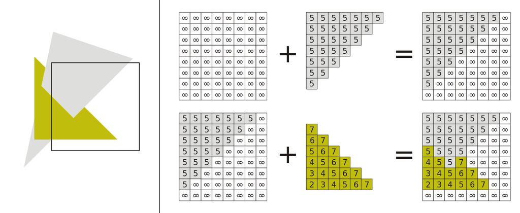
83 Incremental linear evaluation A linear (affine, really) function on the plane is: Linear functions are efficient to evaluate on a grid: 65

84 Incremental linear evaluation lineval(xm, xm, ym, ym, cx, cy, ck) { // setup auto qrow = cx*xm + cy*ym + ck; } // traversal for(auto y : range(ym, ym)) { auto qpix = qrow; for(auto x : range(xm, xm)) { output(x, y, qpix); qpix += cx; } qrow += cy; } cx =.005; cy =.005; ck = 0 (image size 100x100) 66

85 Rasterizing triangles 1. evaluation of linear functions on pixel grid 2. functions defined by parameter values at vertices 3. using extra parameters to determine fragment set 67

86 Defining parameter functions To interpolate parameters across a triangle we need to find the cx, cy, and ck that define the (unique) linear function that matches the given values at all 3 vertices We can solve as a linear system of 3 equations for 3 unknowns: (each states that the function agrees with the given value at one vertex) Leading to a 3x3 matrix equation for the coefficients: (singular iff triangle is degenerate) 68

87 Defining parameter functions More efficient version: shift origin to (x0, y0) q(x, y) = c x (x x 0 ) + c y (y y 0 ) + q 0 q(x 1, y 1 ) = c x (x 1 x 0 ) + c y (y 1 y 0 ) + q 0 = q 1 q(x 2, y 2 ) = c x (x 2 x 0 ) + c y (y 2 y 0 ) + q 0 = q 2 Now this is a 2x2 linear system (since q0 falls out): Solve using Cramer s rule (see Shirley): 69

88 Defining parameter functions lininterp(xm, xm, ym, ym, x0, y0, q0, x1, y1, q1, x2, y2, q2) { // setup det = (x1 x0)*(y2 y0) (x2 x0)*(y1 y0); cx = ((q1 q0)*(y2 y0) (q2 q0)*(y1 y0)) / det; cy = ((q2 q0)*(x1 x0) (q1 q0)*(x2 x0)) / det; qrow = cx*(xm x0)+cy*(ym y0)+q0; // traversal (same as before) for(auto y : range(ym, ym)) { auto qpix = qrow; for(auto x : range(xm, xm)) { output(x, y, qpix); qpix += cx; } qrow += cy; } } 70

89 Interpolating several lininterp(xm, xm, ym, ym, n, x0, y0, q0[], x1, y1, q1[], x2, y2, q2[]) { // setup for(auto k : range(0, n 1)) { // compute cx[k], cy[k], qrow[k] // from q0[k], q1[k], q2[k] // traversal for(auto y : range(ym, ym)) { for(auto k : range(1, n)) qpix[k] = qrow[k]; for(auto x : range(xm, xm)) { output(x, y, qpix); for(auto k : range(1, n)) qpix[k] += cx[k]; } for(auto k : range(1, n)) qrow[k] += cy[k]; } } 71

90 Rasterizing triangles 1. evaluation of linear functions on pixel grid 2. functions defined by parameter values at vertices 3. using extra parameters to determine fragment set 72

91 Clipping to the triangle Interpolate three barycentric coordinates across the plane recall each barycentric coord is 1 at one vert. and 0 at the other two Output fragments only when all three are > 0. 73

92 Pixel-walk (Pineda) rasterization Conservatively visit a superset of the pixels you want Interpolate linear functions Use those functions to determine when to emit a fragment 74

93 Rasterizing triangles Exercise caution with rounding and arbitrary decisions Need to visit these pixels once But it s important not to visit them twice! 75

94 Clipping Rasterizer tends to assume triangles are on screen particularly problematic to have triangles crossing the plane z = 0 After projection, before perspective divide clip against the planes x, y, z = 1, 1 (6 planes) primitive operation: clip triangle against axis-aligned plane 76

95 Clipping a triangle against a plane 4 cases, based on sidedness of vertices all in (keep) all out (discard) one in, two out (one clipped triangle) two in, one out (two clipped triangles) 77

96 Hidden Surface Removal 78

97 Pipeline VERTS. INDICES TRANSFORMED VERTICES ASSEMBLED PRIMITIVES PIXEL FRAGMENTS SHADED FRAGMENTS FINAL IMAGE VERTEX PROCESSING PRIMITIVE ASSEMBLY RASTERIZATION FRAGMENT PROCESSING FRAMEBUFFER PROCESSING Transform vertices and projection Assemble vertices into primitives Fragment generation Lighting z-buffer Compositing 79

98 Hidden surface elimination We have discussed how to map primitives to image space projection and perspective are depth cues occlusion is another very important cue 80

99 Painter s algorithm Simplest way to do hidden surfaces Draw from back to front, use overwriting in framebuffer [WikimediaCommons] 81

100 Painter s algorithm Simplest way to do hidden surfaces Draw from back to front, use overwriting in framebuffer 82

101 Painter s algorithm Simplest way to do hidden surfaces Draw from back to front, use overwriting in framebuffer 82

102 Painter s algorithm Simplest way to do hidden surfaces Draw from back to front, use overwriting in framebuffer 82

103 Painter s algorithm Simplest way to do hidden surfaces Draw from back to front, use overwriting in framebuffer 82

104 Painter s algorithm Simplest way to do hidden surfaces Draw from back to front, use overwriting in framebuffer 82

105 Painter s algorithm Simplest way to do hidden surfaces Draw from back to front, use overwriting in framebuffer 82

106 Painter s algorithm Amounts to a topological sort of the graph of occlusions But when the graph has cycles, no sort is valid [WikimediaCommons] 83

107 The z buffer In many (most) applications maintaining a z sort is too expensive changes all the time as the view changes many data structures exist, but complex Solution: draw in any order, keep track of closest object at pixel allocate extra channel per pixel to keep track of closest depth when drawing, compare object s depth to current closest depth and discard if greater this works just like any other compositing operation Another example of a memory-intensive brute force approach that works and has become the standard 84

108 The z buffer [WikimediaCommons] 85

109 Precision in z buffer Z precision is distributed between the near and far clipping planes this is why these planes have to exist also why you can t always just set them to very small and very large distances Generally use z (not world z) in z buffer 86

110 Interpolating in projection linear interp. in screen space linear interp. in world (eye) space 87

111 Interpolating in projection linear interp. in screen space linear interp. in world (eye) space 87

112 Interpolating in projection linear interp. in screen space linear interp. in world (eye) space 87

113 Interpolating in projection linear interp. in screen space linear interp. in world (eye) space 87

114 Interpolating in projection linear interp. in screen space linear interp. in world (eye) space 87

115 Interpolating in projection linear interp. in screen space linear interp. in world (eye) space 87

116 Interpolating in projection linear interp. in screen space linear interp. in world (eye) space 87

117 Minimal Pipeline Example 88

118 Pipeline for minimal operation Vertex stage (input: position / vtx; color / tri) transform position (object to screen space) pass through color Rasterizer pass through color Fragment stage (output: color) write to color planes 89

119 Result of minimal pipeline 90

120 Pipeline for basic z buffer Vertex stage (input: position / vtx; color / tri) transform position (object to screen space) pass through color Rasterizer interpolated parameter: z (screen z) pass through color Fragment stage (output: color, z ) write to color planes only if interpolated z < current z 91

121 Result of z-buffer pipeline 92

122 Flat shading Shade using the real normal of the triangle Leads to constant shading and faceted appearance [Foley et al.] 93

123 Pipeline for flat shading Vertex stage (input: position / vtx; color and normal / tri) transform position and normal (object to eye space) compute shaded color per triangle using normal transform position (eye to screen space) Rasterizer interpolated parameters: z (screen z) pass through color Fragment stage (output: color, z ) write to color planes only if interpolated z < current z 94

124 Result of flat-shading pipeline 95

125 Transforming normal vectors Transforming surface normals differences of points (and therefore tangents) transform OK normals do not --> use inverse transpose matrix 96

126 Transforming normal vectors Transforming surface normals differences of points (and therefore tangents) transform OK normals do not --> use inverse transpose matrix 96

127 Gouraud shading Compute colors at vertices using vertex normals Interpolate colors across triangles [Foley et al.] 97

128 Pipeline for Gouraud shading Vertex stage (input: position, color, and normal / vtx) transform position and normal (object to eye space) compute shaded color per vertex transform position (eye to screen space) Rasterizer interpolated parameters: z (screen z); r, g, b color Fragment stage (output: color, z ) write to color planes only if interpolated z < current z 98

129 Result of Gouraud shading 99

130 Local vs. infinite viewer, light Phong illumination requires geometric information: light vector (function of position) eye vector (function of position) surface normal (from application) Light and eye vectors change per vertex 100

131 Local vs. infinite viewer, light Look at case when eye or light is far away: distant light source: nearly parallel illumination distant eye point: nearly orthographic projection in both cases, eye or light vector changes very little Optimization: approximate eye and/or light as infinitely far away 101

132 Directional light Light vector always points in the same direction many pipelines are faster if you use directional lights 102

133 Directional light Light vector always points in the same direction many pipelines are faster if you use directional lights 102

134 Infinite viewer Orthographic camera: projection direction is constant Infinite viewer : even with perspective, we can approximate eye vector using the image plane normal 103

135 Non-diffuse Gouraud shading Can apply Gouraud shading to any illumination model Results are not so good for specular shading [Foley et al.] 104

136 Per-pixel (Phong) shading Get higher quality by interpolating the normal just as easy as interpolating the color but now we are evaluating the illumination model per pixel rather than per vertex (and normalizing the normal first) in pipeline, this means we are moving illumination from the vertex processing stage to the fragment processing stage 105

137 Per-pixel (Phong) shading Bottom line: produces much better highlights [Foley et al.] 106

138 Pipeline for per-pixel shading Vertex stage (input: position, color, and normal / vtx) transform position and normal (object to eye space) transform position (eye to screen space) pass through color Rasterizer interpolated parameters: z (screen z); r, g, b color; x, y, z normal Fragment stage (output: color, z ) compute shading using interpolated color and normal write to color planes only if interpolated z < current z 107

139 Result of per-pixel shading 108

140 Antialiasing 109

141 Aliasing continuous image defined by ray tracing procedure continuous image defined by a bunch of black rectangles 110

142 Rasterizing lines Define line as a rectangle Specify by two endpoints Ideal image: black inside, white outside 111

143 Rasterizing lines Define line as a rectangle Specify by two endpoints Ideal image: black inside, white outside 111

144 Point sampling Approximate rectangle by drawing all pixels whose centers fall within the line Problem: all-or-nothing leads to jaggies This is sampling with no filter (aka. point sampling) 112

145 Point sampling Approximate rectangle by drawing all pixels whose centers fall within the line Problem: all-or-nothing leads to jaggies This is sampling with no filter (aka. point sampling) 112

146 Point sampling 113

147 Aliasing Point sampling is fast and simple But the lines have stair steps and variations in width This is an aliasing phenomenon: sharp edges of line contain high frequencies Introduces features to image that are not supposed to be there! 114

148 Antialiasing Point sampling makes an all-or-nothing choice in each pixel therefore steps are inevitable when the choice changes yet another example where discontinuities are bad On bitmap devices this is necessary hence high resolutions required 600+ dpi in laser printers to make aliasing invisible On continuous-tone devices we can do better 115

149 Antialiasing Basic idea: replace is the image black at the pixel center? with how much is pixel covered by black? Replace yes/no question with quantitative question. 116

150 Box filtering Pixel intensity is proportional to area of overlap with square pixel area Also called unweighted area averaging 117

151 Box filtering by supersampling Compute coverage fraction by counting subpixels Simple and accurate But slow 118

152 Box filtering 119

153 Weighted filtering Box filtering problem: treats area near edge same as area near center results in pixel turning on too abruptly Alternative: weight area by a smooth function unweighted averaging corresponds to using a box function a gaussian is a popular choice of smooth filter important property: normalization (unit integral) 120

154 Weighted filtering Compute filtering integral by summing filter values for covered subpixels Simple, accurate But really slow 121

155 Weighted filtering Compute filtering integral by summing filter values for covered subpixels Simple, accurate But really slow 121

156 Gaussian filtering 122

157 Filter comparison Point sampling Box filtering Gaussian filtering 123

158 Supersampling vs. multisampling Supersampling is terribly expensive GPUs use an approximation called multisampling Compute one shading value per pixel Store it at many subpixel samples, each with its own depth 124

159 Multisample rasterization Each fragment carries several (color,depth) samples shading is computed per-fragment depth test is resolved per-sample final color is average of sample colors single- sample multi- sample [ 125

160 Antialiasing textures With multisampling, we evaluate textures once per fragment Need to filter the texture somehow since perspective produces high minification Solution: render textures with one (few) samples/pixel but filter them first [Akenine-Möller et al. 2008] 126

161 Solution: pixel filtering point sampling area averaging [Akenine-Möller et al. 2008] 127

162 Pixel footprints image space texture space [Akenine-Möller et al. 2008] 128

163 Pixel vs. texels Optimal viewing distance: one-to-one mapping between pixel area and texel area When closer, magnification: each pixel is a small part of the texel When farther, minification: each pixel includes many texels [Akenine-Möller et al. 2008] upsampling magnification downsampling minification 129

164 Filter size by Jacobian image space texture space (0,1) ( u y, v ) y ( u x, v ) x (1,0) y x v ψ(x) x u 130

165 Mipmap pyramid MIP Maps: (Multum in Parvo) Store a hierarchy of pre-filtered versions of texture While rendering, use the version with texel size closer to pixel size [Akenine-Möller et al. 2002] 131

166 Compute Mipmaps Average over 4x4 neighbors or use Gaussian filtering Storage increase by 33% [WikimediaCommons] 132

167 Point sampling 133

168 Point sampling 133

169 Gaussian filtering 134

170 Gaussian filtering 134

171 Mipmap filtering 135

172 Mipmap filtering 135

173 Lighting with Textures 136

174 Lighting In rasterization, no access to the geometry during shading significantly better efficiency, parallelism, memory locality Shadows need occluder information Reflections need recursive evaluation Option 1: drop pipeline done in offline rendering, not any time soon for real-time Option 2: cheat the lighting use approximate, or even plainly wrong, alsorithms run data multiple times through the pipeline 137

175 Shadow mapping Pass 1: Render from the light, store z buffer as a depth texture Pass 1: Render from eye, check if distance to the light computed in fragment shader is less then the one saved in the depth texture [NVisia Cg Tutorial] 138

176 Shadow mapping Render from light Store z-buffer in shadow map Render from eye [WikimediaCommons] Project shadow map Test if shadow map closer than light Multiply by color for final image 139

177 Shadow mapping artifacts Pixelation due to mismatched resolution [Fernando et al.] 140

178 Shadow mapping artifacts [Fernando et al.] Pixelation due to mismatched resolution 141

179 Reflection mapping [M. C. Escher] [Paul Debevec] 142

180 Reflection mapping Pass 1-6: Render from object center into a 360 panorama using 6 cameras arranged as a cube often store as cube map Pass 7: Render from eye, look up the texture in mirror direction [Paul Haeberly] 143

181 Reflection mapping Pass 1-6: Render from object center into a 360 panorama using 6 cameras arranged as a cube often store as cube map [WikimediaCommons] 144

182 Reflection mapping artifacts Geometric distortions: works only at the center of projection Visibility is missing: reflect what it should not [WikimediaCommons] 145