Minimizing Edge Length to Connect Sparsely Sampled Unstructured Point Sets

Transcription

1 Minimizing Edge Length to Connect Sparsely Sampled Unstructured Point Sets Stefan Ohrhallinger a,b, Sudhir Mudur a, Michael Wimmer b a Concordia University, Montréal b Vienna University of Technology Abstract Most methods for interpolating unstructured point clouds handle densely sampled point sets quite well but get into trouble when the point set contains regions with much sparser sampling, a situation often encountered in practice. In this paper, we present a new method that provides a better interpolation of sparsely sampled features. We pose the surface construction problem as finding the triangle mesh which minimizes the sum of all triangles longest edge. Since searching for matching umbrellas among sparsely sampled points to yield a closed manifold shape is a difficult problem, we introduce suitable heuristics. Our algorithm first connects the points by triangles chosen in order of their longest edge and with the requirement that all edges must have at least 2 incident triangles. This yields a closed non-manifold shape which we call the Boundary Complex. Then we transform it into a manifold triangulation using topological operations. We show that in practice, runtime is linear to that of the Delaunay triangulation of the points. Source code is available online. 1. Introduction Defining the piece-wise linear boundary shape for a solid object in R 3, for which only the surface point coordinates but nothing of its connectivity is known, is a difficult problem. It has been the subject of a lot of research over the last 3 decades. Unorganized point sets are increasingly encountered resulting from simulations of objects with connectivity changing over time, or editing, e.g. with particles or sketches. Scanning techniques may supply the connectivity partly though not reliably, say in the form of estimated normals, contours, or overlaps from different perspectives. However, Hoppe et al argue very well the need for solving this problem as a generic one [1]. The generic problem we wish to solve is strict interpolation of all the given points in a point set, a problem of theoretical and practical interest. The point set is assumed to be reasonably densely sampled in most regions but could still contain smaller regions which are much more sparsely sampled. This situation is quite common, since obtaining uniformly dense sampling is difficult in practice. Figure 1 compares results from a few well known methods using a sparsely sampled Stanford bunny. As we wish to accurately interpolate such more sparsely sampled regions also, we consider all given points, even in these regions, as features and not as outliers or noise. For point sets with noise such as those resulting from non-high fidelity sensing devices, use of our method would require prior denoising with an appropriate noise model. Surface fitting, the alternative approach in which densely sampled features are usually reconstructed, tends to smooth over sharp features (see some examples in Figure 14 later), whereas retention of sharp corners and fine features is the main concern of this work. Hence we shall limit the discussion in this paper mainly to interpolating methods. We show nevertheless that our method is quite robust in handling point data which would normally be considered as noisy. (a) Wrap (c) Shrink (b) TightCocone (d) Our method Figure 1: Comparing reconstruction of a sparsely sampled Stanford bunny using different methods: a) Wrap, b) TightCocone, c) Shrink, with d) Our method, which interpolates it with a connected, oriented and water-tight boundary. Preprint submitted to Computer & Graphics May 28, 2013

2 lated are quite restrictive, in order to permit a unique surface to interpolate the points. This makes it hard to find real-world data sets fulfilling them. However, the reconstruction methods presented actually work for some point sets well outside these conditions. This is made possible by employing suitable heuristics or (potentially slow) searching. We therefore believe that it is of greater relevance to empirically compare the output from implementations, rather than just their guaranteed (but far more restrictive) sampling conditions. Figure 2: The method in R 2 [2] which we use as base. Left: The hull of the BC is partially deflated (similar to an air mattress). Center: Adding triangles from DT inflates BC into a polygonal hull. Right: Removing triangles in DT sculptures that hull to interpolate all points. Detecting boundaries (holes) in surfaces, which are commonplace in range data, always requires specifying a threshold for the non-uniformity of the sampling density. In the absence of such specifications, a point set therefore represents an orientable closed surface, which is the generic problem we address in this paper. Detection and handling of boundaries is thus not considered as being within the scope of this paper. The problem of connecting unorganized points into a boundary shape has been extensively addressed in R 2 with the goal of recognizing shapes. A recent method presented in [2] has successfully addressed the reconstruction of a closed interpolated boundary from extremely sparse samples. They exploit Gestalt principles. In R 3 it is even more complex to find a shape in the form of an interpolating oriented surface, bounding a volume. We extend the approach in [2] (see Figure 2) into R 3. Our experiments show that the resulting water-tight surface is also aesthetically pleasing which we attribute again to our objective of following the Gestalt principles. The major claims in this paper are: We define a perception-inspired minimization objective which enables us to connect, with an orientable closed surface, more sparsely sampled point sets than earlier methods. We introduce the Boundary Complex, an extension of the Minimum Spanning Tree into R 3. As an application it provides us a good starting set to efficiently obtain a closed interpolating surface for reasonably dense sampled point sets. We propose topological operations, which transform the boundary complex into a closed manifold triangulation. We present an extended algorithm, with suitable heuristics which avoid exhaustive searching. It extracts an orientable closed surface for point sets with small regions containing much sparser point sets, as commonly encountered in practical examples. Previous methods have given sampling conditions, based on uniformity or local feature size [3]. These conditions as formu Related Work Based on the three-dimensional Delaunay triangulation of the points, the concept of α-shapes was introduced in the seminal paper by Edelsbrunner and Mücke [4]. This formulation requires a globally uniform parameter, which leads to a tradeoff between loss of detail and hole filling. This work is extended in [5] with a γ-neighborhood graph that adapts locally to variable point density, however the method is not robust. An advancing-front algorithm based on α-shapes is introduced in [6], but it also fails for non-uniformly spaced point sets. The method was extended to locally non-uniform sampling, but does not interpolate all points [7]. Further, since advancing front algorithms depend on seed triangles, their results are not deterministic. Boissonnat estimates at each given point a local tangent plane using nearby points and then determines the local neighborhood by projecting those points on that plane [8]. He assigns points as neighbors based on an angle criterion. In [9] natural neighbors are derived from the Delaunay triangulation projected on such a plane. For both methods, a plane is fit using the k-nearest neighbors. Using a single value for k globally has the disadvantage that for many points this value will either be too small or too large to give suitable local support. Where these neighbors are distributed anisotropically, the resulting normal will not be representative. The more recent method [10] based on theoretical guarantees of [11] for uniformly sampled point sets suffers from the same problem. They require prior extraction of a dense uniformly sampled point set whose quality depends again on the estimation of the underlying surface. The method in [12] creates umbrellas locally at the vertices from the set of Gabriel triangles. It uses topological postprocessing to match these umbrellas and fill holes by solving a system of integer linear inequalities, but this becomes very slow with increase in the number of sparsely spaced points. This method guarantees the surface to be water-tight, but does not optimize any aspect of the surface. Further these inequalities lead to undesired disconnection of some of the surface components. Our use of heuristics to handle sparse regions certainly presents a computation time advantage over their work. Another method in [13] creates umbrellas for a selected subset of points and then re-inserts unprocessed points. This work does not guarantee an orientable surface, contrary to our requirement of a water-tight oriented surface. Boissonnat introduced, in a second approach in that paper [8], the technique of sculpturing. He mentions a proof

3 that any polyhedron of genus 0 can be extracted from the convex hull by removing tetrahedra in the Delaunay triangulation, based on certain heuristic rules. Since this is also of combinatorial complexity, he proposed a greedy algorithm which removes such tetrahedra sorted by an intrinsic criterion. However, the method can end up quickly in local minima and may therefore miss interpolating many of the given points. Further, the resulting shape is restricted to a genus of 0. The method in [14] constrains sculpturing such that Gabriel triangles are not removed from the boundary. It detects and creates holes in the object (genus > 0) where edges in the Euclidean Minimum Spanning Tree span non-neighbor vertices on its boundary, but the object can become hollowed out at under-sampled regions. Surface tension is used as a criterion for a variant of sculpturing in [15]. While its results seem visually pleasing for surfaces permitting boundaries, constraining it to output a water-tight surface yields artifacts for more sparse sampling, such as connecting distant parts of the surface or disconnecting parts of the boundary. In our method we start the sculpturing process with an initial triangle set, which already represents a water-tight boundary close to the output surface. This leads to better results as we shall see in the many examples discussed later. Amenta et al [3] were the first to guarantee homeomorphic surface reconstruction (their Crust algorithm), for an ɛ-dense sampling in proportion to medial axis distance, where ɛ=0.1. This sampling condition is extremely stringent, permitting only very blunt dihedral angles (an averaged 166 ) at the edges, in order to be able to fit a surface uniquely. This crust is extracted by locally filtering the Delaunay complex, although it may contain many slivers and needs post-processing to extract the actual surface triangles in order to produce the manifold. The Power Crust algorithm is presented in [16] which reconstructs under-sampled regions better, but introduces many additional points. In [17] the original Crust is simplified to the Cocone algorithm. Later in [18] it is extended to their TightCocone algorithm which fills holes, provided the under-sampling is local. While water-tightness is thus guaranteed, for more sparse sampling, it often disconnects boundary parts, or discards them as not contained on or interior to the boundary. In a follow-up paper [19], in a method called RobustCocone, filtering of the restricted Delaunay complex is proposed to remove noisy points, which are not clearly oriented outside or inside its envelope, but this results in loss of fine features. Both [20] and [21] use flow to classify the critical points of a distance function, in order to restrict the Delaunay complex. While the flow complex is well established, and performs well in reconstructing surfaces with boundaries, its given guarantees to extract a closed manifold homeomorphic to the sampled surface ( [22], [23]) do not surpass previously given ones, or refer only to the weaker homotopy [24]. Besides in [20] it is mentioned that the computation of the flow complex is of (possibly much) higher order than the Delaunay complex. In [25] the witness complex is used to extract an interpolating surface from noisy point sets. In relation to earlier methods, our focus is to guarantee water-tightness while trying to achieve strict interpolation of the given points. In one of the first attempts to use an optimization approach 3 Petitjean and Boyer use an initial set of Gabriel triangles and then select triangles by minimal circumradius to extract a manifold [26]. In [27] the problem is formulated as a graph cut by weighting approximate visibility and minimizing the longestto-shortest ratio of edges in triangles, but they require carefully optimized parameters to be specified for every point set. In [28] a global algorithm which minimizes a criterion for the surface and analyzes different heuristics is proposed. It extends the edge length criterion from R 2 to correspond to area or circumradius of triangles in R 3. But the heuristic of inserting triangles to fulfill the constraint of 2 triangles per edge, as well as its proposed dual, get very easily stuck in local minima, yielding sub-optimal results. In our approach, we also pursue the goal of energy minimization but combine it successfully with a closely approximating starting set, requiring heuristics only for more sparsely sampled regions. Our experiments show that TightCocone [18] and Shrink [15] yield good results among other previous work for our specific problem, namely, interpolating point sets representing sparsely sampled surfaces with a guaranteed closed manifold. Wrap [21] and also Shrink give good results if a closed manifold is not required. 3. Overview of Our Proposed Approach We propose first that there exists a surface, well-defined by minimizing an energy functional, forming the boundary shape for a given point set. We propose further that while we cannot always guarantee its exact construction, we can approximate it well, depending on a time-budget. There may be point sets which are much too sparse or highly non-uniformly spaced for which humans also cannot easily see the boundary shape. But we maintain that the class of point sets with not too sparse or not too non-uniform sampling is still much larger than the classes which previous methods can reconstruct. By assuming such a surface, every given point set has a shape whose form is bounded by the connectivity of that surface. We can then construct that shape boundary, or for overly sparse sampling, select an acceptable approximation (using suitable heuristics), which is still a closed manifold surface, and thus improve upon the results of earlier comparable methods. For this, we introduce a generic hole-filling technique and extend the well-known technique of sculpturing with a dual called inflating (see Figure 3). The rest of the paper is organized as follows. In Section 4 we define the minimum boundary of the shape, a closed interpolating manifold surface which minimizes an objective. Next, we relax its topological constraint to define the minimum boundary complex. In Section 5 we describe the basic algorithm, which transforms the minimum boundary complex for sufficiently dense sampling into a closed manifold boundary while maintaining the minimization objective. In Section 6, we follow this with an extension of the algorithm to handle locally more sparsely sampled point sets. In Section 7 we present varied examples of constructed surfaces and compare our results with some of the earlier algorithms, together with run-times. We present a brief discussion on some significant aspects of

4 Converting to Manifold Hull Sculpturing u>=1 Boundary Complex: BC 0 u=0 or u=1 Manifold Hull: H(BC) u=1 Interpolating Manifold: B out Figure 3: Our method in a nutshell. Left: Triangles in the BC which form artifacts are colored grey (slivers) or red (hull holes). Center: Hole covering and inflating transforms the BC into a polyhedral hull. Right: Sculpturing exposes an interior polyhedron which interpolates all points. our method in Section 8 and follow it with our conclusions in Section 9 along with the various potential extensions. 4. Minimum Boundary and a Fast Approximation Let P in three-dimensional Euclidean space R 3 denote the given unorganized point set. Let DT(P) (or DT for short) denote the Delaunay triangulation of the point set P with all its elements in R 3. We assume with a small loss of generality that P is in general linear position to avoid degenerate cases of DT. We define a triangulation as manifold if each vertex not on its boundary is also manifold, i.e. forms the center of exactly one closed triangle fan, which we name an umbrella. Such a manifold triangulation also has exactly two incident triangles for each interior edge, making those manifold as well. Boundary edges are those that have only one incident triangle. We call a triangulation that has no boundary edges a polyhedron. A polyhedron is, by definition, a closed manifold surface Minimum Boundary Surface (B min ) Let B denote a polyhedron that interpolates all p P. We further impose the constraint B DT, which ensures that triangles do not self-intersect and also helps reducing computational complexity. We call B the set of such closed sub-manifolds of DT interpolating P. Then B min B is the one that minimizes the intrinsic criterion of B that is discussed next. In order to find B min, we need to minimize a criterion based on its geometric primitives Choosing a Suitable Criterion To be able to evaluate the criterion for a single primitive (point, edge or triangle), we require it to be self-contained. An example in R 2 is edge length, and minimizing the total length of the boundary shape has shown to yield good results [29]. We therefore try to extend this to R 3. Several triangle measures 4 (a) Circumradius (b) Aspect ratio (c) Area (d) Longest edge Figure 4: Comparing surface minimization criteria selfcontained in a triangle. We chose d) Longest edge. could be considered for this, including area, circumradius, inradius, longest side, perimeter, aspect ratio, etc. We have evaluated these measures (see Figure 4) by plugging them into Algorithm 1 presented later in Sub-section 4.3. Using area or inradius produces many long, thin triangles, which tend to connect non-neighbor regions of the point set. The circumradius gives good results in general, but replaces even small triangles having two near-collinear vertices (since circumradius tends to infinity) by such long, thin triangles. To avoid these problems, we minimize the longest edge in a triangle and, as we see later in Section 7, this yields excellent results. One advantage is that this criterion is already reflected in the underlying triangulation DT, through its property of maximizing its minimum angle, thus leading to short edges. Accordingly we define our measurable criterion for an individual triangle t as: λ(t) = max e (1) e t Now we give the complete definition for the minimum boundary: B min = argmin B B λ(t) (2) In the above equation, we have chosen to minimize sum of λ. An alternative is to minimize average λ. However, since we never actually compute the minimum in our algorithm, but t B

5 (a) u=1 (b) u=2 (c) u=1 (d) u=2 Figure 5: The u-valence is the number of umbrellas at a vertex of the graph or triangulation: a, b) In R 2 the inside of the boundary is shaded yellow. c, d): R 3. (a) BC 0 (b) Output surface B out only approximate it by ordering triangles by their λ, this is not relevant for its final result Minimum Boundary Complex (BC min ) A naive approach of determining B min would be to iterate through all possible B B and choosing the one that minimizes Equation (2). Enumerating all 2 n combinations of triangles in a DT with n triangles is NP-hard. Even determining a manifold with local topological post-processing can become slow or infeasible for non-trivially sized point sets, as mentioned in [12]. Therefore, B min could only be constructed for trivial point sets. In order to solve the corresponding problem in R 2, the Minimum Boundary Complex BC min was introduced in [2], where a vertex is allowed to have 2 incident edges (instead of exactly 2 as for B min in 2D), while also keeping the same minimization objective. They then show its use for efficient construction of B min or its close approximation. We note that we can also define an umbrella in R 2. It consists of 2 edges incident to a vertex and then vertices with 2 incident edges have 1 umbrellas (see Figure 5). This permits us to generalize BC min in both R 2 and R 3 as relaxing the number umbrellas from u = 1 (B min ) to u 1. Thus, we can formally define the Minimum Boundary Complex (BC min ) in R 3 as follows: Definition 1. Let BC DT be a connected set of triangles spanning the point set P such that each vertex v BC has 1 umbrellas in BC, and let BC be the set of all thus defined triangle sets. Then, BC min is defined as BC min = argmin BC BC 4.4. Boundary Complex BC 0 λ(t). (3) t BC Unfortunately, as in R 2, exact computation of BC min is also difficult in R 3. Still, its relaxed connectivity constraint enables us to construct a close approximation using the greedy Algorithm 1 with run-time proportional to DT construction (see Table 2). We call the output of this greedy construction algorithm BC 0, since it is not guaranteed to be minimal. Algorithm 1 constructs BC 0 BC by considering triangles from DT sorted by ascending λ(t i ). A triangle is added to BC 0 under any of the following conditions: Figure 6: Yellow triangles represent the large overlap between: a) BC 0 (artifacts shaded grey). b) Result of our method B out. it is incident to a vertex not in BC 0 (to span all points), it is incident to a boundary edge in BC 0, it connects two connected components in BC 0. The algorithm produces a unique result, provided triangles of equal λ(t) in DT are sorted lexicographically. Further, it is also guaranteed not to contain any boundary edges, a property which will prove useful in the topological operations defined later. Input: P, DT Output: BC 0 PQ := priority-queue of t i DT, sorted by λ(t i ); Remove first t 0 from PQ; BC 0 := {t 0 }; while (BC 0 is not a connected component) ( (v P) BC 0 ) ( boundary edge e i BC 0 ) do Remove first t i from PQ; if (t i connects unconnected triangles in BC 0 ) (t i connects to a boundary edge e i BC 0 ) ( (v t i ) BC 0 ) then Insert t i into BC 0 ; foreach boundary edge e j t i do Insert all {t j e j t j, t j DT, t j BC 0 } into PQ; end end end Algorithm 1: Construction of BC 0 Requiring at least two incident triangles per edge and connectedness yields global closure. If we omit the last condition of connectedness, then we only get local closure. This permits multiple boundary components, e.g. for distant components. BC 0 is a very good shape approximation because its triangles overlap largely with those in B out (see Figure 6). This is due to the fact that the only difference in definition is the slightly relaxed topological constraint. This overlap BC 0 B out can be identified easily: vertices in BC 0 with u = 1 are very likely to be interpolated by that same umbrella in B out, since the triangles in BC 0 are selected by the same minimization criterion. 5

6 5. Making the Approximated Boundary Manifold Our goal is to transform BC 0 into a closed manifold boundary B out, while maintaining the same minimization objective. Intuitively, points sampled on a smooth surface S can be connected well to their neighbors if those have shorter Euclidean distance than any samples on distant surface parts. The boundary complex captures this well by filtering triangles with short edges from DT. The above intuition can be expressed formally by sufficiently dense sampling with respect to local feature size, which for a point x S is the Euclidean distance of x to its closest point in the medial axis M [30]. The medial axis M for a smooth surface S is the closure of all points in R 3 with 2 closest points in S [31]. It is well known that the DT of even arbitrarily dense sampled point sets contain slivers, i.e., flat tetrahedra which are elongated along the surface, since its four vertices are nearcoplanar (see examples in Figure 7). These slivers cause BC 0 to exhibit two types of (offending) artifacts (detailed in the next sub-section) which should not be present in B out, the closed manifold boundary. Our experiments have shown that most practical models lack sufficiently dense sampling only in small regions and that overall, the required sampling is not required to be highly dense, as is demanded by many earlier proposed methods. We will show first in this section that under the assumption of sufficiently dense sampling, the topological properties of BC (the term which we will use generically, for BC 0 and its subsequent alterations) make transformation to a B out quite simple. Then in Section 6, we will extend this basic algorithm to handle regions with extremely sparse sampling Overview The two types of artifacts (see Figure 7) are: hullhole (a) Hull-hole (b) Covered hull-hole (c) Sculptured (d) 2D cross-section (e) 2D cross-section (f) 2D cross-section (g) Sliver set Figure 7: Artifacts in BC: a) A hull-hole (shaded black), bounded by four sliver tetrahedra in BC (shaded red), which in turn are partitioned by an artifact boundary L (black lines) from the remaining manifold triangulation (shaded yellow). b) Hole-covering has added the lid (two triangles) in place of the hull-hole to complete the disk triangulation bounded by L. c) Sculpturing has removed redundant triangles from the slivers to transform the artifact and merge it into a manifold boundary. d- f) 2D cross-sections corresponding to figures in the upper row. g) Sliver set: Two tetrahedra (shaded red) share the triangle bde. Sliver sets: BC contains all four triangles of a sliver tetrahedron, as two pairs of triangles, each pair connected with an obtuse dihedral angle. Since its four vertices in BC are not manifold, we have to remove one triangle pair. To generalize, we refer either to a single sliver or to a number of slivers, if they share triangles in DT, as a sliver set. Hull holes: The greedy construction of BC may result in its triangulation folding back onto itself, skipping triangles with larger λ(t). This folding back causes holes in the hull of BC. The hull is the connected set of outer triangles, more precisely defined later in Section 5.2. Contrary to what we do for sliver sets in BC, for this type of artifact we have to add those skipped triangles. Hull holes are always bounded by (sets of) slivers adjacent to edges where the triangles fold back. These edges make up the edgeboundary of the hull-hole. On the other hand, a hole in a non-zero genus manifold mesh, e.g. a donut, would not have such an edge-boundary. hull hole (a) Artifacts hull hole (b) L 0 is genus 0 hull hole (c) L 1 is genus 1 Figure 8: Hull hole detection: a) Hull-hole (in center) bounded by slivers (shaded red) and a separate sliver (shaded grey), separated by edges with 2 incident triangles (dotted) from the manifold triangulation (yellow). b) L 0 bounds the single separate sliver. c) L 1 bounds the sliver set containing the hull hole. We apply the following four steps to fix these artifacts, thus transforming BC into B out : 6

7 (a) H(BC) with deflated entities (b) Manifold H(BC) Figure 9: 2D example illustration (representative for 3D) of edges in DT (solid if also in BC, with its interior shaded yellow). H(BC) is determined as the subset of BC reachable from the convex hull (outside edges) by traversing adjacent triangles without passing through edges in BC. a) An oriented (cyclic) traversal of H(BC) encounters some entities in BC (red) twice, we name those deflated. b) H(BC) with no deflated entities. Locate artifact boundaries as oriented edges, so as to contain all non-manifold entities (i.e., those incident to vertices with u > 1) onto a specific side of that artifact boundary. After the subsequent steps of artifact transformation, only bounded manifold triangulations remain, which can then be stitched together by those artifact boundaries. Detect hull holes in artifacts by checking if there does not exist a triangulated disk in BC bounded by the edgeboundary of the artifact and on its inside. Cover hull holes by adding triangle sets to BC so as to convert these artifacts also into sliver sets. Since all edgeboundaries of artifacts then bound a manifold triangulation inside, after this step there will exist a B out BC. Remove slivers by applying an extension of the sculpturing technique given in [8] to remove all slivers from BC, resulting in a B out. We have observed that for sufficiently dense sampling, hull holes are rare and both types of artifacts are locally contained (see Figure 6). Below we discuss significant aspects of each of the above four steps to make clear all the issues involved in their implementation Locate Artifact Boundaries in BC We first need to partition BC into triangle subsets which are either artifacts or bounded manifold triangulations (see Figure 8). We require of such a partitioning edge-boundary that it splits the BC into two disjoint subsets and define a sub-set of BC which contains all of them, next. A traversible hull of BC. Artifacts in BC may overlap where slivers share triangles. But we are able to define an oriented (cyclic) traversal on a set of triangles T DT, which then form its hull H(T). H(T) T is the triangle set reachable from the triangles on the convex hull of P by traversing adjacent tetrahedra in DT without passing through triangles in T (see Figure 9 for a 2D illustration). H(BC) then refers to the hull of BC. Edge-boundaries must split BC. Any edge-boundary which partitions BC into two disjoint subsets of triangles must be an 7 orientable edge-chain and be contained in H(BC). Such an edge-boundary is also contained in B out, since it is only through its edges that the triangle subsets can reach each other. Determining artifact boundaries. Edges in H(BC) which bound an artifact must have > 2 incident triangles since BC by definition has no boundary edges nor can such an edge be interior to a manifold triangulation. We extract all orientable edge-chains L which consist of such edges with > 2 incident triangles (with exactly 2 of those in H(BC) incident at its inside), as the artifact boundaries Detect Artifacts with Hull-Holes Artifacts are polyhedra. For each artifact, the previous step yields its artifact boundary L and its set of triangles T. Since edges in L have 2 incident triangles in H(BC) on the inside of the artifact with respect to L, H(T) is a polyhedron and L forms a loop in its hull. Hull Holes are polyhedra of non-zero genus. If L partitions H(T) into two subsets such that they only share L, then H(T) is of genus zero and H(BC) contains two manifold triangulations bounded by L, namely those two subsets. Otherwise H(T) is a polyhedron of non-zero genus, containing hull holes (see Figure 8). Determining non-zero genus. We start from an edge in L and traverse edge-connected triangles in H(T) once and until an edge in L is encountered. If any edge in L is traversed twice, the artifact is of non-zero genus Cover Hull-Holes with Lids Many lids may exist. Now we have to find a set of triangles to add to a non-zero genus artifact such that its hull becomes of genus zero. As an example, a hull hole of genus one resembles a donut, so we have to find a triangulated disk closing the hole, which we call a lid. Many oriented edge loops may exist in H(T), each bounding one or more lids. Instead of exhaustively searching the above-mentioned space for a lid, we will determine a triangle set which is guaranteed to contain all lids, as shown next. Then we merge it with BC and leave it to the sculpturing step to extract the boundary triangles. Determining the triangle set containing all lids. Let V be the set of all vertices in T, the artifact triangle set. The boundary complex computed for the point set V, namely BC(V), consists of triangles with all their vertices in V. It follows that all disks of triangles in DT, which are bounded by L and whose vertices are contained in V, are contained in BC(V). Therefore, merging BC(V) with BC converts the artifact into a sliver set. Doing this for all artifacts with hull holes will make H(BC) manifold Remove Slivers by Sculpturing Since the resulting hull H(BC) contains a bounded manifold triangulation at each side for all artifact boundaries, it is a polyhedron and as such a B out. However, BC, which may still contain slivers and therefore is not a manifold, could contain a polyhedron even closer to our minimization objective, so we want to extract that instead.

8 (a) Interior vertex (b) Exposed vertex (c) Flipped edge Figure 10: Sculpturing [8] rules. a) Tetrahedron q 0 with single boundary triangle. b) Removal of q 0 exposes its interior vertex p. c) Removal of q 1 flips edge e to e. Boissonnat [8] originally introduced the sculpturing algorithm to extract a manifold boundary interpolating a point set from its convex hull as follows: Sculpturing rules. A tetrahedron q can be removed from a manifold hull H DT by toggling its triangles in H if it satisfies either of the following (see Figure 10): (a) From H(DT) (b) From H(BC 0 ) I(BC 0 ) Figure 11: Sculpturing with λ(t): a) Result by sculpturing directly from the convex hull boundary - a large hole in the bottom leads to a hollowing-out of the object. b) Much improved result by sculpturing from the manifold hull of the boundary complex using our method. 3 vertices, 3 edges and 1 triangle in H: exposes the vertex of the tetrahedron which is interior to H (this case does not occur for the results from our basic algorithm). 4 vertices, 5 edges and 2 triangles in H: flips an edge in H to remove a sliver tetrahedron from H. Disadvantages of the original sculpturing algorithm. Since it starts from the convex hull it often runs into local minima, particularly for sparse point sets. It also cannot produce non-zero genus objects. Since H(BC) has a manifold boundary, we can apply sculpturing to it. Further, from our experiments we have found that removing tetrahedra only from outside of the H(BC) tends to hollow it out. To retain the minimization objective, we add an inside equivalent of the hull boundary to be sculptured, with the same rules. Sculpturing from in- and outside. Since P samples S sufficiently densely and BC after the addition of lids only contains slivers and no interior vertices, there exists an inside hull I(BC) BC, similar to its outside hull H(BC). We determine the set of polyhedra inside H(BC) which do not contain triangles of BC in their interior. I(BC) is then the largest of these inside polyhedra (all others represent sliver sets). We use the triangle set H(BC) I(BC) for sculpturing. Hulls of BC are a better starting set. H(BC) and I(BC) are both a much closer approximation to B out than the convex hull and also permit boundaries of genus > 0. The example in Figure 11 compares the results, which also holds for the examples shown later. 6. Extended Algorithm for Increased Sparsity We extend our basic algorithm (Figure 12) to handle problems caused by even more sparse sampling, which is common in small regions of many point sets in practice. For that, we need the following definition: 8 Figure 12: The steps of our extended algorithm in order, preceded by sub-section numbers. We call an entity (vertex, edge or triangle) in H(BC) deflated if it is encountered more than once during a cyclic traversal of H(BC) (see Figure 9). Intuitively, this happens when pinching an inflatable object from two sides such that finger tips (vertex), hand sides (edge) or flat hands (triangle) meet Orientable Artifacts The first problem which can occur is that all artifact boundaries may not be orientable as is required by our basic algorithm. For the artifacts to be orientable, BC must conform to the following conditions: Each deflated edge must separate its connected triangles in H(BC) by tetrahedra exterior to H(BC) in exactly two sides, named inside and outside. Each deflated vertex must contain all its incident deflated edges in a single umbrella in H(BC), which guarantees

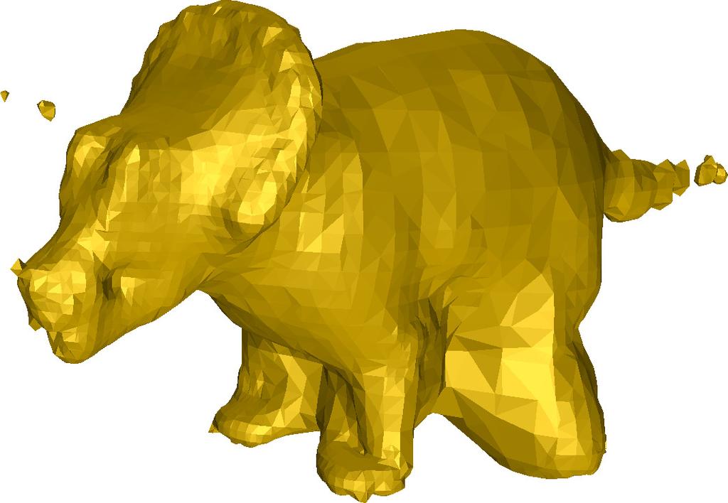
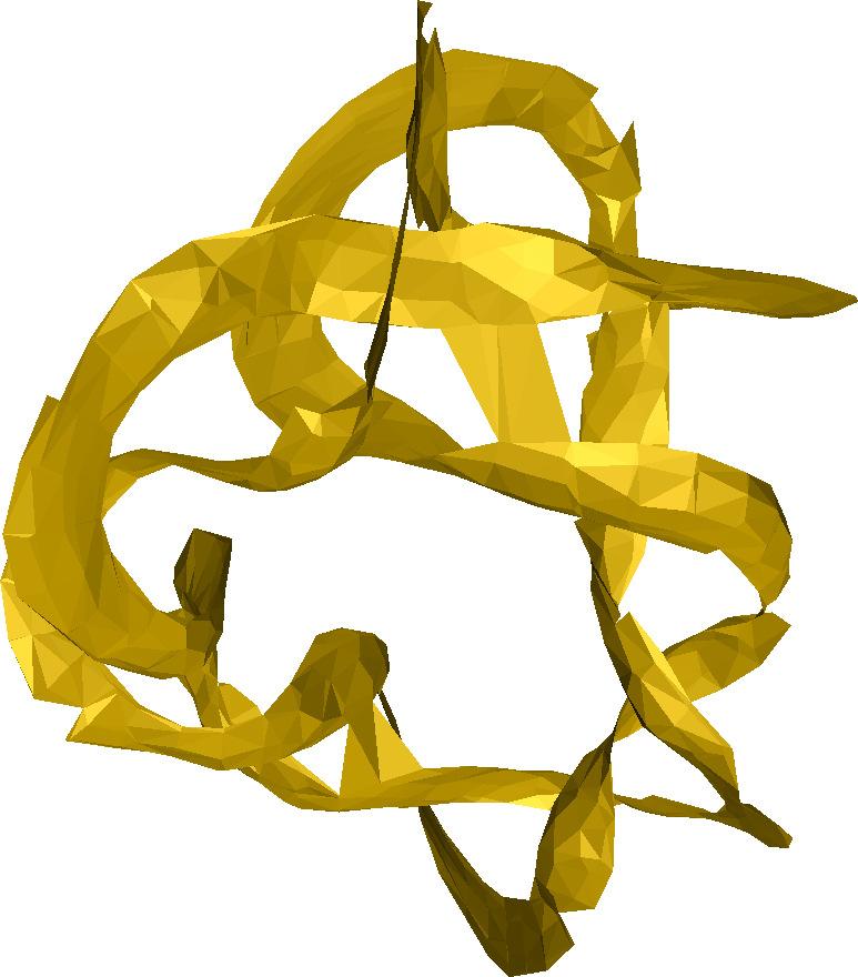
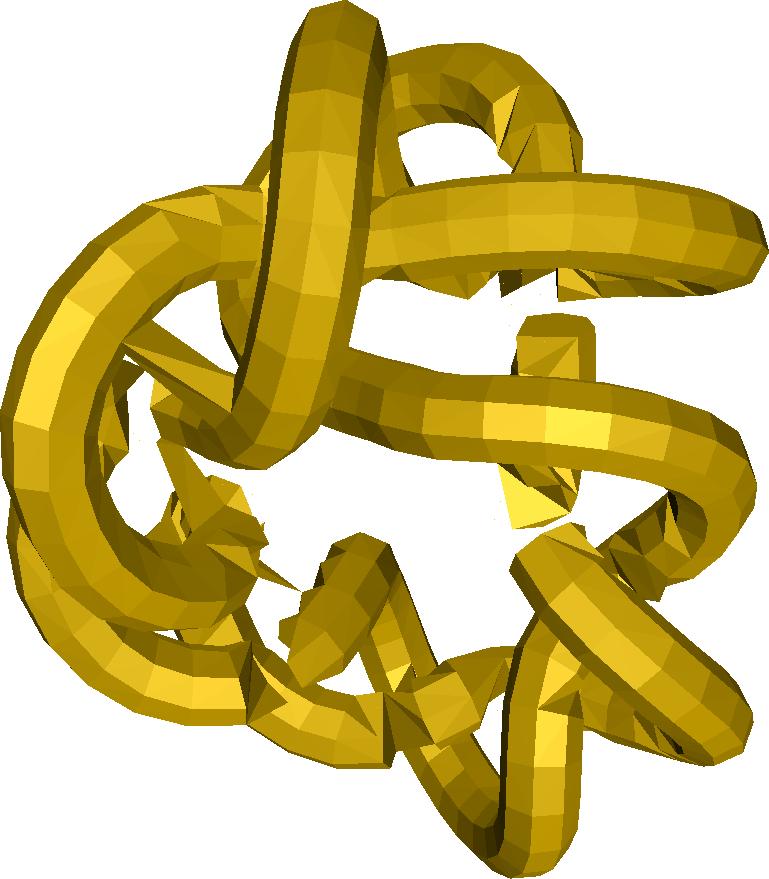
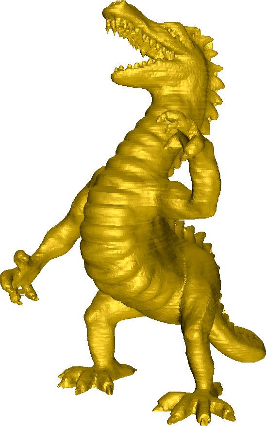
9 that connected deflated edges form a planar graph, so that loops of deflated edges in H(BC) are orientable. Deflated vertices must be contained in deflated edges, since our basic algorithm assumes artifact boundaries to consist only of edges. Note that there may exist deflated edges which are contained in hull-hole artifacts and not in its boundary. Therefore deflated edges do not generally form oriented edge-chains in H(BC) (see Figure 8c), but those belonging to artifact boundaries can still be found by simple traversal with back-tracking. In our experiments, we found only a small number of entities (vertices and edges) not conforming to these conditions. To transform those into conforming entities, we inflate selectively (add tetrahedra), ordered by our minimization criterion. We repeat this process until all these entities (and any entities which have become non-conforming by adding tetrahedra) become conforming. The latter case happens only rarely, as we have seen in our experiments, so the operation converges quickly to yield a conforming BC Inflating The second problem is that even after adding lids to hullholes, deflated entities may remain in H(BC), which is then not manifold. This is because, with highly sparse sampling, BC 0 may connect distant surface parts to each other, the way opposite sides of any not fully inflated air mattress may touch. We introduce a dual operation to sculpturing, inflating, which transforms BC such that H(BC) becomes a closed manifold surface. For this we add tetrahedra to it which are in DT and outside of H(BC), as illustrated in R 2 in Figure 2. The algorithm for inflating is given below: Inflating Algorithm. Let V o denote the set of deflated vertices in the hull H(BC). A tetrahedron q DT exterior to H(BC) is a candidate for adding if it contains 1 vertices in V o and 1 triangles in H(BC). Input: BC, V o Output: BC (has manifold hull) PQ := priority-queue of candidates q, sorted by λ(t) where t {t q, t q t H(BC)}; while PQ {} do Remove first tetrahedron q i from PQ; BC:=BC q i ; foreach q j DT exterior to H(BC) sharing a vertex with q i do Determine if q j is a candidate and update PQ with it; end end BC := BC; Algorithm 2: Inflating Mitigation of Getting Trapped in Local Minima The third problem is that for very sparse sampling, even inout sculpturing can get trapped in a local minimum. This happens when tetrahedra get removed for which their triangle with smallest circumradius is located in the hull. To mitigate this, we add a rule which prohibits removal of such tetrahedra. As a consequence, BC may retain some sliver sets after sculpturing. But we are still able to extract a manifold from these extreme cases, which also interpolates all points, except possibly some points in regions with very high sparsity. 7. Results Name Vert DT Total Dey s Shrink int curv Torus 0.2k 0.02s 0.7s 0.04s 0.05s 0 1% Bunny 0.5k 0.02s 0.14s 0.08s 0.02s 0 1% Knot 1k 0.06s 0.27s 0.14s 0.04s 0 0% Triceratops 3k 0.14s 1.07s 0.74s 0.21s 0 2% Bowl 3k 0.17s 2.67s 0.62s 0.13s 3 3% Mechpart 4k 0.18s 1.35s 1.1s 0.18s 0 4% Mannequin 13k 0.45s 3.75s 3.36s 0.47s 0 3% Pegasus 14k 1.71s 9.25s 6.08s 0.74s 564 3% Dragon 54k 3.58s 19.29s 22.36s 3.44s 14 4% Dinosaur 65k 3.88s 17.56s 22.64s 3.7s 0 4% Armadillo 172k 10.45s 60.86s 71.2s 9.41s 0 5% Table 1: Runtime for our entire surface reconstruction algorithm (non-optimized implementation), with proportion of Delaunay triangulation construction, and compared to TightCocone, on a single 2.67Ghz 64bit AMD CPU. Actual complexity for our method seems to decrease with model size compared to TightCocone but is not as fast as Shrink. The number of interior (non-interpolated) vertices in B are also given, to see whether a point set is in class C u (int=0). TightCocone fails to interpolate far more points than our algorithm does. Post-processing reduces absolute mean curvature by curv. Name DT BC 0 Inflate Hole Sculpt Mannequin 12% 15% 38% 19% 15% Pegasus 19% 6% 27% 16% 30% Dragon 19% 15% 34% 19% 13% Dinosaur 22% 13% 35% 17% 10% Armadillo 17% 16% 33% 19% 12% Table 2: Proportional timings for the steps of our algorithm, for the larger models, in order: Delaunay triangulation construction, boundary complex, inflating, segmentation, hole-covering and sculpturing. Our algorithm is implemented in C++, using the CGAL library [32] for the construction of the Delaunay triangulation and a Disjoint set library [33]. Source code is provided [34]. Improved quality. In Figure 13 we show examples with some very sharp corners, like in the right-most sub-figure. In Figure 14, taking a few more examples of somewhat more challenging point sets (since more sparse), we compare our method with an approximating method, Poisson [35], and the following interpolating methods: Wrap [21], which has no water-tight

10 (a) Mannequin, 13k (b) Armadillo, 172k (c) Dinosaur, 65k (d) Mechpart, 4k (e) Torus, 0.2k (f) Basic Figure 13: a-e): Example results of our reconstruction methods along with point set sizes. f): It should be noted that the three point sets, regular tetrahedron, cube and polyhedron with 16 faces cannot be reconstructed by TightCocone. guarantee, and TightCocone [18] and Shrink [15] which do have that. We use default parameters for all methods. From the above figures it is clear that Poisson as a fitting method can not deal well with sharp corners. Wrap algorithm manages to interpolate most of the points, but is only able to generate flat, bounded triangulations for the sparsely sampled regions, which may also result in holes. In such sparsely sampled regions, TightCocone and Shrink disconnect components, create undesired connections and TightCocone fails to interpolate many points. Our method is more robust, resulting in fewer undesired connections (e.g. Bowl between bottom and stem in Figure 14) or holes in thin structures (e.g. the Pegasus wings in Figure 14), where sampling is extremely sparse. Competitive runtime. We show in Table 1 that our algorithm (non-optimized implementation) has nevertheless competitive run-time compared with TightCocone [18], even if slower than Shrink and that it is proportional to that of the Delaunay triangulation construction. Details of the time taken for the steps of our method are listed in Table 2. Since these only need to operate on subsets of the entire Delaunay triangulation, we expect the run-time of an optimized implementation to be smaller than its construction. 8. Discussion of Our Method (a) Original (b) 0.1% perturbed (c) 0.3% perturbed (e) -14% (f) -19% (g) -38% (d) perturbed 1% (h) -70% Figure 16: Row 1 demonstrates robustness to noise (and local non-uniformity) of our method by perturbing the coordinates of the points with uniform noise (percentage relative to z-extent of point set). c) the noise level exceeds point distances in the fine features such as the eyes. Row 2 reconstructs the surface with RobustCocone [36]: Note that its smoothing, while approximating differential quantities like normals or curvature better, results in dropping many points (percentages given below the figures). Thus it removes not only outliers but also features, as can be seen already in the original point set (mouth, eyes, ear). Guarantees for the output surface Bout : All points are guaranteed to be interpolated on or interior to Bout, unlike TightCocone, since BC0 spans P and points are never disconnected outside Bout. The majority of points in the input point set are interpolated entirely (see Table 1). Bout is guaranteed to be a single connected component, due to the component-connectedness condition of Algorithm 1. If desired otherwise, this condition can simply be dropped, then permitting multiply connected boundaries. Bout is always manifold and water-tight, as a result of the hole-filling and inflating steps. 10

11 no result Figure 14: Comparing original point sets (row 1), Poisson (row 2), Wrap (row 3), TightCocone (row 4), Shrink (row 5) with our method (row 6), for varied point sets with extremely non-dense or non-uniform subsets; note the poor results of the other methods for thin structures. The results of TightCocone and our method are water-tight, whereas the results of Poisson and Wrap are not. 11

12 (a) Stanford Bunny (b) 23% sub-sampled (c) 5% sub-sampled (d) 1% sub-sampled (e) 0.3% sub-sampled (f) 0.1% sub-sampled Figure 15: Robustness to non-dense point sets is demonstrated by the Stanford bunny keeping its shape well, when down-sampling from the original 36k to just 33 points. (a) Failure case (b) 2D cross-section (c) Inflating failure Figure 17: a) The hull hole boundary (around non-scanned bottom) is twisted such that there does not exist a single disk in DT covering it. Inflating to obtain a water-tight boundary would then add those undesired triangles. b) 2D cross-section showing the split disk (dotted lines). c) Same with inflated result. Based on a proof for 2D in [2], which we believe is extensible into R 3, we conjecture that sufficiently dense sampling required for our basic algorithm is ɛ < 0.5, significantly higher than the best currently known result of ɛ < 0.1 in [3]. Limitations: Twisted holes: Our method cannot cover a hull hole, for which no lid entirely made up by vertices of the slivers inside its artifact boundary exists, e.g. if a distant part of the surface penetrates the hole (a possible case for extremely sparse sampling). As a consequence, the inflating step will fall into a local minimum. However, we believe that labeling triangles in BC outside the artifact boundary as in- or outside would permit similar hole filling as described in [18]. In practice, we have observed this only in scans which completely omitted the bottoms, as seen in Figure 17. Advantages: Robustness to down-sampling: That shapes for non-dense point sets are robustly constructed by our method is well illustrated in Figure 15. All of the other above-mentioned methods fare poorly for this extremely sparse point set (Stanford bunny down-sampled, up to a factor of 1000). 12 Tolerance to noise: The tolerance of our method for construction from noisy point sets is demonstrated in Figure 16, for point coordinates perturbed with random uniform noise of up to 10 times the feature size (average point distance). It retains the fine features and interpolates most points, while RobustCocone [36] smooths over those features uniformly, dropping many points. Close to minimum absolute mean curvature: We found that a post-processing step, which flips edges to locally minimize absolute mean curvature, will only change it by very little (see Table 1), showing that λ(t) correlates well with it. Easy shape visualization: The boundary complex BC 0 is non-manifold, but closely approximates the final shape. This enables us to display the shape boundary for visualization purposes by just rendering the result of the simple Algorithm 1. As the starting set for the reconstruction method, it also handles sparse and noisy point sets very well. Dense sampling should yield B out = B min : We conjecture that for sufficiently dense sampling such that no edges in BC 0 intersect the medial axis of the smooth surface S, the basic algorithm produces B min. Because B min minimizes λ(t), any triangles removed by edge-flipping would have larger λ(t), since they connect to further neighbors. 9. Conclusion and Future Work The strength of our method is its ability to extract watertight surfaces from much sparser sampling than earlier methods. This is made possible by (i) our imposition of the closure property, which as we know is true for physical objects, i.e. its (triangulated) surface has no boundaries, and (ii) our formulation of the minimum boundary complex, which provides us with a really good initial shape approximation, based on the longest-edge-in-triangle criterion. We felt it was more important to show that the proposed minimization solution adequately fulfills the reconstruction goal and further that this minimum is approximated well. Fortunately, our results also show that this combinatorial search space is still quite manageable where sampling quality is such that humans

13 can still recognize the shape boundary well. Proving a better sampling condition would, as in previous methods, be of more theoretical interest. The fundamental contributions in our work permit to expand it in various directions, of which we list a few: Surfaces with boundaries. By specifying a parameter for a local non-uniformity threshold, hull hole artifacts could be marked and their surface boundary extracted through sculpturing rather than covering it. Optimal topological mesh repair. Self-inter-secting triangles can be removed as not in DT and completing the BC 0 removes boundary edges not belonging to a mesh boundary. Continuing our method then would generically remove all topological artifacts, without requiring to handle specific cases and would produce a water-tight triangulation, minimizing our objective. Neighborhood computation. The edges in BC 0 incident to a vertex represent well its nearest neighbors since the artifacts do not affect edge connectivity. Contrary to k-nearest neighbors, it does not require a global parameter and may yield more faithful normals. Real-time visualization. Although DT-based methods are relatively slow, ours could be employed for visualizing point clouds as meshing-on-demand in the view frustum, by doing deterministic local umbrella matching for densely sampled points in parallel. Resampling. If we resample a given surface sufficiently dense to conform to our basic algorithm, not only this may reduce the number of points required to represent it, but allows to drop the connectivity entirely. This has applications in compression or shape retrieval. Since the resampling operator is local, it can also be adapted to out-of-core construction. References [1] H. Hoppe, T. DeRose, T. Duchamp, J. McDonald, W. Stuetzle, Surface reconstruction from unorganized points, Computer Graphics 26 (2) (1992) [2] S. Ohrhallinger, S. Mudur, An efficient algorithm for determining an aesthetic shape connecting unorganized 2d points, computer Graphics Forum, to appear (2013). [3] N. Amenta, M. Bern, Surface reconstruction by voronoi filtering, Discrete and Computational Geometry 22 (1998) [4] H. Edelsbrunner, E. P. Mücke, Three-dimensional alpha shapes, in: VVS 92: Proceedings of the 1992 workshop on Volume visualization, ACM, New York, NY, USA, 1992, pp [5] R. C. Veltkamp, Boundaries through scattered points of unknown density, Graph. Models Im. Proc. 57 (6) (1995) [6] F. Bernardini, J. Mittleman, H. Rushmeier, C. Silva, G. Taubin, The ballpivoting algorithm for surface reconstruction, IEEE Trans. on Vis. and Comp. Graph. 5 (4) (1999) [7] D. Cohen-Steiner, F. Da, A greedy delaunay-based surface reconstruction algorithm, Vis. Comput. 20 (1) (2004) [8] J.-D. Boissonnat, Geometric structures for three-dimensional shape representation, ACM Trans. Graph. 3 (4) (1984) [9] M. Gopi, S. Krishnan, C. Silva, Surface reconstruction based on lower dimensional localized delaunay triangulation, Computer Graphics Forum 19 (3) (2000) [10] D. Dumitriu, S. Funke, M. Kutz, N. Milosavljevic, How much Geometry it takes to Reconstruct a 2-Manifold in r 3, in: Proceedings of the 10th Workshop on Algorithm Engineering and Experiments, ALENEX 2008, San Francisco, USA, ACM-SIAM, San Francisco, USA, 2008, pp [11] S. Funke, E. A. Ramos, Smooth-surface reconstruction in near-linear time, in: SODA 02: Proc. of the 13th annual ACM-SIAM symp. on Discrete algorithms, SIAM, Philadelphia, PA, USA, 2002, pp [12] U. Adamy, J. Giesen, M. John, Surface reconstruction using umbrella filters, Comput. Geom. Theory Appl. 21 (1) (2002) [13] G. Kós, An algorithm to triangulate surfaces in 3d using unorganised point clouds, in: Geometric Modelling, Springer-Verlag, London, UK, 2001, pp [14] M. Attene, M. Spagnuolo, Automatic surface reconstruction from point sets in space, CG Forum 19 (3) (2000) [15] R. Chaine, A geometric convection approach of 3-d reconstruction, in: SGP 03: Proceedings of the 2003 Eurographics/ACM SIGGRAPH symposium on Geometry processing, Eurographics Association, Aire-la- Ville, Switzerland, 2003, pp [16] N. Amenta, S. Choi, R. Kolluri, The power crust, unions of balls, and the medial axis transform, Computational Geometry 19 (2001) (27). [17] N. Amenta, S. Choi, T. K. Dey, N. Leekha, A simple algorithm for homeomorphic surface reconstruction, in: SCG 00: Proc. 16th ann. symp. Computat. geometry, ACM, New York, NY, USA, 2000, pp [18] T. K. Dey, S. Goswami, Tight cocone: a water-tight surface reconstructor, in: SM 03: Proceedings of the eighth ACM symposium on Solid modeling and applications, ACM, New York, NY, USA, 2003, pp [19] T. K. Dey, S. Goswami, Provable surface reconstruction from noisy samples, in: Proceedings of the 20th annual symposium on Computational geometry, SCG 04, ACM, New York, NY, USA, 2004, pp [20] J. Giesen, M. John, The flow complex: a data structure for geometric modeling, in: Proceedings of the fourteenth annual ACM-SIAM symposium on Discrete algorithms, SODA 03, Society for Industrial and Applied Mathematics, Philadelphia, PA, USA, 2003, pp [21] H. Edelsbrunner, Surface Reconstruction by Wrapping Finite Sets in Space, Discrete and Computational GeometryThe Goodman-Pollack Festschrift 25 (1) (2003) [22] T. K. Dey, J. Giesen, E. A. Ramos, B. Sadri, Critical points of the distance to an epsilon-sampling of a surface and flow-complex-based surface reconstruction, in: Proceedings of the 21st annual symp. on Computational geometry, SCG 05, ACM, New York, NY, USA, 2005, pp [23] E. A. Ramos, B. Sadri, Geometric and topological guarantees for the wrap reconstruction algorithm, in: Proceedings of the 18th annual ACM-SIAM symposium on Discrete algorithms, SODA 07, Society for Industrial and Applied Mathematics, Philadelphia, PA, USA, 2007, pp [24] B. Sadri, Manifold homotopy via the flow complex, Computer Graphics Forum 28 (5) (2009) [25] L. Guibas, S. Oudot, Reconstruction using witness complexes, Discrete & Computational Geometry 40 (2008) [26] S. Petitjean, E. Boyer, Regular and non-regular point sets: Properties and reconstruction, Comput. Geom. Theory Appl. 19 (2001) [27] P. Labatut, J.-P. Pons, R. Keriven, Robust and efficient surface reconstruction from range data, Comp. Graphics Forum 28 (8) (2009) [28] H. Hiyoshi, Optimization-based approach for curve and surface reconstruction, Comput. Aided Des. 41 (2009) [29] S. Ohrhallinger, S. P. Mudur, Interpolating an unorganized 2d point cloud with a single closed shape, Computer-Aided Design 43 (12) (2011) [30] J. Ruppert, A new and simple algorithm for quality 2-dimensional mesh generation, in: Proc. 4th ann. ACM-SIAM Symposium on Discrete algorithms, SODA 93, SIAM, Philadelphia, PA, USA, 1993, pp [31] H. Blum, A Transformation for Extracting New Descriptors of Shape, in: W. Wathen-Dunn (Ed.), Models for the Perception of Speech and Visual Form, MIT Press, Cam., 1967, pp [32] S. Hert, M. Seel, dd convex hulls and Delaunay triangulations, in: CGAL User/Ref. Man., 3.8 Edition, CGAL Ed. Board, [33] E. Stefanov, Disjoint Sets Data Structure Implementation, (2011 (accessed May 13, 2011)). [34] S. Ohrhallinger, D. Prieler, Source-code of algorithm in this paper, (May 2013). [35] M. Kazhdan, M. Bolitho, H. Hoppe, Poisson surface reconstruction, in: Proc. 4th Eurographics symp. on Geometry processing, SGP 06, Eurographics Association, Aire-la-Ville, Switzerland, 2006, pp [36] T. K. Dey, S. Goswami, Provable surface reconstruction from noisy samples, Computational Geometry: Theory and Appl. 35 (1) (2006)