Digital Image Processing. Week 4

Transcription

1

2 Morphological Image Processing Morphology deals with form and structure. Mathematical morphology is a tool for extracting image components that are useful in the representation and description of region shape, such as boundaries, skeletons, and the convex hull. In this chapter, the inputs are binary images but the outputs are attributes extracted from these images. A i j I i, j {(, ); 1(white)} 2

3 Preliminaries The reflection of a set B, denoted B is defined as B { w ; w b, for b B } The translation of a set B by point z = (z1, z2), denoted (B)z is defined as ( B) { c; czb for b B } z

4 Set reflection and translation are used in morphology to formulate operations based on so-called structuring elements (SE): small sets or subimages used to probe an image under

5 study for properties of interest. In addition to a definition of which elements are members of the SE, the origin of a structuring element also must be specified. The origin of the SE is usually indicated by a black dot. When the SE is symmetric and no dot is shown, the assumption is that the origin is at the center of symmetry. When working with images, it is required that structuring elements are rectangular arrays. This is accomplished by

6 appending the smallest possible number of background elements necessary to form a rectangular array.

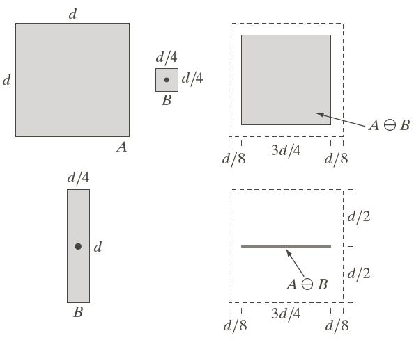
7 Erosion and Dilation Digital Image Processing Many of the morphological algorithms are based on these two primitive operations: erosion and dilation. Erosion Let A and B be to sets from denoted A B is defined as: A B { z ; ( B) A } 2. The erosion of A by B, This definition indicates that the erosion of A by B is the set of all points z such that B, translated by z, is contained in A. z

8 In the following, set B is assumed to be a structuring element. Because the statement that B has to be contained in A is equivalent to B not shearing any common elements with the background, erosion can be expressed equivalently: c A B { z ; ( B) A } z

9

10 Equivalent definitions of erosion: 2 A B{ w ; wba for every bb } A B ( A) b Erosion shrinks or thins objects in a binary image. We can view erosion as a morphological filtering operation in which image details smaller than the structuring element are filtered (removed) from the image. bb

11 Dilation Let A and B be to sets in A B is defined as: Digital Image Processing 2. The dilation of A by B, denoted A B{ z ; ( B) A } The dilation of A by B is the set of all displacements z, such that B and A overlap by at least one element. We assume that B is a structuring element. Equivalent definitions of dilation: 2 A B{ w ; w ab, for some aa and bb } z

12 A B ( A) b The basic process of rotating B about its origin and then successively displacing it so that it slides over set (image) A is analogous to spatial convolution. Dilation being based on set operations is a nonlinear operation, whereas convolution is a linear operation. Unlike erosion which is a shrinking or thinning operation, dilation grows or thickens objects in a binary image. The bb

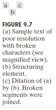
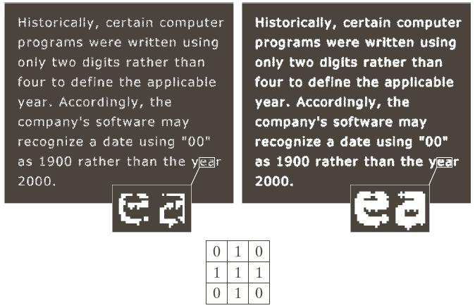
13 specific manner and the extent of this thickening are controlled by the shape of the structuring element used. One of the simplest applications of dilation is for bridging gaps.

14

15 Duality Erosion and dilation are duals of each other with respect to set complementation and reflection: A B A B c c c c A B A B The duality property is useful particularly when the structuring element is symmetric with respect to its origin, so that B B. Then, we can obtain the erosion of an image by B simply by dilating its background (i.e. dilating A c ) with the same structuring element and complementing the result.

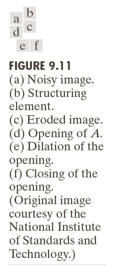
16 Opening and Closing Opening generally smoothes the contour of an object, breaks narrow isthmuses, and eliminates thin protrusions. Closing also tends to smooth section of contours but, as opposed to opening, it generally fuses narrow breaks and long thin gulfs, eliminates small holes, and fills gaps in the contour.

17 The opening of set A by structuring element B is defined as: A B A B B Thus, the opening of A by B is the erosion of A by B, followed by a dilation of the result by B. Similarly, the closing of set A by structuring element B is defined as: AB A B B which says that the closing of A by B is the dilation of A by B, followed by an erosion of the result by B.

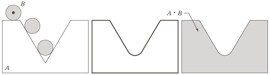
18 The opening operation has a simple geometric interpretation. Suppose that we view the structuring element B as a (flat) rolling ball. The boundary of A B is then established by the points in B that reach the farthest into the boundary of A as B is rolled around the inside of this boundary. The opening of A by B is obtained by taking the union of all translates of B that fit into A. A B {( B), za;( B) A } z z

19 Closing has a similar geometric interpretation, except that now we roll B on the outside of the boundary.

20

21

22 Opening and closing are dual of each other with respect to set complementation and reflection: c c AB A B c c A B A B The opening operation satisfies the following properties: 1. A B A 2. if C D then CB D B 3. AB B A B

23 Similarly, the closing operation satisfies the following properties: 1) A AB 2) if C D then CB DB 3) AB B A B Condition 3 in both cases states that multiple openings or closings of a set have no effect after the operator has been applied once.

24

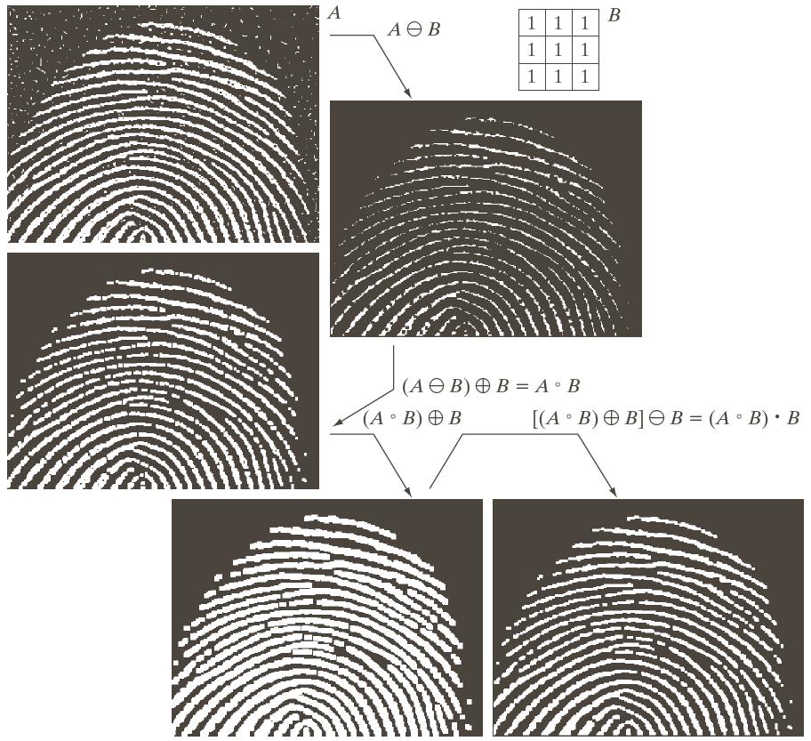
25 The Hit-or-Miss Transformation The morphological hit-or-miss transformation is a basic tool for shape detection. Consider the set A from Figure 9.12 consisting of three shapes (subsets) denoted C, D, and E. The objective is to locate one of the shapes, say, D. Let the origin of each shape be located at its center of gravity. Let D be enclosed by a small window, W. The local background of D with respect to W is defined as the set difference (W-D) (Figure 9.12(b)). Figure 9.12(c) shows the

26 complement of A. Fig. 9.12(d) shows the erosion of A by D. Figure 9.12(e) shows the erosion of the complement of A by the local background set (W-D). From Figures 9.12(d) and (e) we can see that the set of location for which D exactly fits inside A is the intersection of the erosion of A by D and the erosion of A c by (W-D) as shown in Figure 9.12(f). If B denotes the set composed of D and its background, the match (or the set of matches) of B in A, denoted A B is: c AB ( AD) A ( W D)

27

28 We can generalize the notation by letting B = (B1, B2), where B1 is the set formed from elements of B associated with an object and B2 is the set of elements of B associated with the corresponding background (B1=D, B2=W-D) in the preceding example). A B AB A B c ( 1) 2 The set A B contains all the (origin) points at which, simultaneously, B1 found a match ( hit ) in A and B2 found a

29 match in A c. Taking into account the definition and properties of erosion we can rewrite the above relation as: A B ( A B ) ( AB ) 1 2 The above three equations for A B are referred as the morphological hit-or-miss transform.

30 Some Basic Morphological Algorithms When dealing with binary images, one of the principal applications of morphology is in extracting image components that are useful in the representation and the description of shape. We consider morphological algorithms for extracting boundaries, connected components, the convex hull, and the skeleton of a region. The images are shown graphically with 1s shaded and 0s in white.

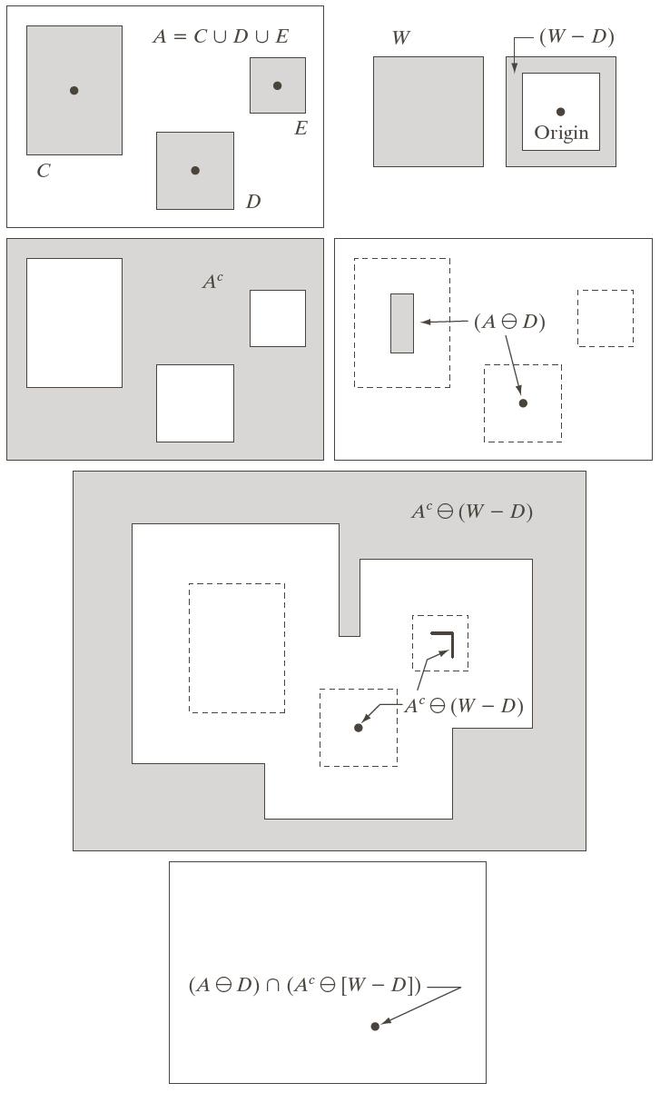
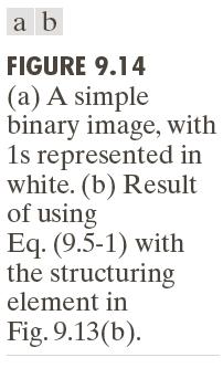
31 Boundary Extraction The boundary of a set A, denoted β(a), can be obtained by first eroding A by B and then performing the set difference between A and its erosion. ( A) A A B where B is a suitable structuring element.

32

33

34 Filling Holes A hole may be defined as a background region surrounded by a connected border of foreground pixels. We present an algorithm based on set dilation, complementation, and intersection for filling holes in an image. Let A denote a set whose elements are 8-connected boundaries, each boundary enclosing a background region (i.e. a hole). Given a point in each hole, the objective is to fill all the holes with 1s.

35 We form an array, X0, of 0s (the same size as the array containing A), except at the location in X0 corresponding to the given point in each hole, which is set to 1. The following procedure fills all the holes with 1s: c Xk Xk1 B A, k 1,2,3,... where B is the symmetric structuring element in Figure 9.15(c). The algorithm terminates at iteration step k if Xk=Xk-1. The set Xk then contains all the filled holes. The set union of Xk and A contains all the filled holes and their boundaries.

36

37 Extraction of Connected Components Extraction of connected components from binary images is important in many automated image analysis applications. Let A be a set containing one or more connected components. Form an array X0 (of the same size as the array containing A) whose elements are 0s (background values), except at each location known to correspond to a point in each connected component in A, which we set to 1

38 (foreground value). The objective is to start with X0 and find all the connected components. The procedure that accomplishes this task is the following: X ( X B) A, k 1,2,3,... k k1 where B is a suitable structuring element. The procedure terminates when Xk = Xk-1, with Xk containing all connected components of the input image.

39

40

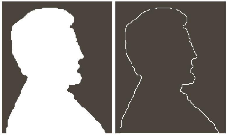
41 Figure 9.18(a) shows an X-ray image of a chicken breast that contains bone fragment. It is of considerable interest to be able to detect such objects in processed food befor packing and/or shiping. In this case, the density of the bones is such that their normal intensity values are different from the background. This makes extraction of the bones from the background a simple matter by using a single threshold. The result is the binary image in Figure 9.18(b). We can erode the thresholded image so that only objects of significant size

42 remain. In this example, we define as significant any object that remains after erosion with a 5 5 structuring elemnt of 1s. The result of erosion is shown in Figure 9.18(c). The next step is to analyse the objects that remain. We identify these objects by extracting the connected components in the image. There are a total of 15 connected components, with four of them being of dominant size. This is enough to determine that significant undesirable objects are containd in the original image.

43 Convex Hull A set A is said to be convex if the straight line segment joining any two points in A lies entirely within A. The convex hull H of an arbitrary set S is the smallest convex set containing S. The set difference H-S is called the convex deficiency of S. Convex hull and convex deficiency are useful for objects description. We present a simple morphological algorithm for obtaining the convex hull C(A) of a set A.

44

45 Let B i, i=1,2,3,4, represent the four structuring elements in Figure 9.19(a). The procedure consists of implementing the equation: X i 0 A X ( X B ) A, i 1,2,3,4 and k 1,2,3,... i i i k k1 i i When the procedure converges ( X k X k 1), we let Then the convex hull of A is 4 C( A) D i1 i D i X. i k

46 The method consists of iteratively applying the hit-or-miss transform to A with B 1 ; when no further changes occur, we perform the union with A and call the result D 1. The procedure is repeated with B 2 (applied to A) until no further chances occur; and so on. The union of the four resulting Ds constitutes the convex hull of A.

47 Thinning, thickening c A BA( AB) A( A B) - thinning B B B B B i is the rotated version of B i {,,, n } 1 2 { i n A B } ( (( AB ) B ) ) B Thickening A B A( AB) 1 2 { i n A B } ( (( AB ) B ) ) B

48

49

50

51

52 Color Image Processing Color Image Processing Color Image Processing Color is very important characteristic of an image that in most cases simplifies object identification and extraction form a scene. Human eye can discern thousands of color shades and intensities and only two dozen shades of gray. Color image processing is divided in 2 major areas: full-color (images acquired with a full-color sensor) and pseudocolor (gray images for which color is assigned) processing.

53 The colors that humans can perceive in an object are determinde by the nature of the light reflected from the object.visible light is composed of a relatively narrow band of frequencies in the electromagnetic spectrum (390nm to750nm). A body that reflects light that is balanced in all visible wavelengths appears white to the observer. A body that favors reflectance in a limited range of the visible spectrum exhibits some shades of color.

54 For example, blue objects reflect light with wavelengths from 450 to 475 nm, while absorbing most of the energy of other wavelengths.

55 How to characterize light? If the light is achromatic (void of color) its only attribute is its intensity (or amount) determined by levels of gray (black-grays-white). Chromatic light spans the electromagnetic spectrum from approximately 400 to 720 nm. Three basic quantities are used to describe the quality of a chromatic light source: radiance, luminance, and brightness.

56 - Radiance is the total amount of energy that flows from the light source (usually measured in watts). - Luminance (measured in lumens lm) gives a measure of the amount of energy an observer percieves from a light source. For example, the light emitted from a source operating in the infrared region of the spectrum could have significant energy (radiance), but an observer would hardly perceive it (the luminance is almost zero).

57 - Brightness is a subjective descriptor, that cannot be measured, it embodies the achromatic notion of intensity and is a factor describing color sensation. Cones are the sensors in the eye responsible for color vision. It has been established that the 6 to 7 million cones in the human eye can be devided into three principal sensing categories, corresponding roughly to red, green, and blue.

58 Approximately 65% of all cones are sensitive to red light, 33% are sensitive to green light, an only about 2% are sensitive to blue (but the blue cones are the most sensitive).

59 Due to these absorbtion characteristics of the human eye, colors are seen as variable combinations of the so-called primary colors : red (R), green (G), and blue (B). For the purpose of standardization, the CIE (Commission Internationale de l Eclairage) designated in 1931 the following specific wavelength values to the three primary colors: blue= nm, green = nm, and red=700 nm. The CIE standards correspond only approximately with experimental data.

60 These three standard primary colors, when mixed in various intensity proportions, can produce all visible colors. The primary colors can be added to produce the secondary colors of light magenta (red+blue), cyan (green+blue), and yellow (red+green). Mixing the three primaries, or a secondary with its opposite primary color in the right intensities produces white light. We must differentiate between the primary colors of light and the primary colors of pigments. A primary color for

61 pigments is one that substracts or absorb a primary color of light and reflects or transmits the other two. Therefore, the primary colors of pigments are magenta, cyan, and yellow, and the secondary colors are red, green, and blue.

62 The characteristics usually used to distinguish one color from another are brightness, hue, and saturation.

63 Brightness embodies the achromatic notion of intensity. Hue is an attribute associated with the dominant wavelength in a mixture of light waves. Hue represents dominat color as percieved by an observer (when we call an object to be red, orange or yellow we refer to its hue). Saturation refers to the relative purity or the amount of white light mixed with a hue. The pure spectrum colors are fully saturated. Color such as pink (red+white) and lavander (violet+white) are less

64 saturated, with the degree of saturation being inversely proportional to the amount of white light added. Hue and saturation taken together are called chromaticity, and therefore a color may be characterized by its brightness and chromaticity. The amounts of red, green, and blue needed to form any particular color are called the tristimulus values and are denoted X, Y and Z, respectively. A color is specified by its trichromatic coefficients, defined as:

65 x y z X X Y Z Y X Y Z Z X Y Z x y z 1

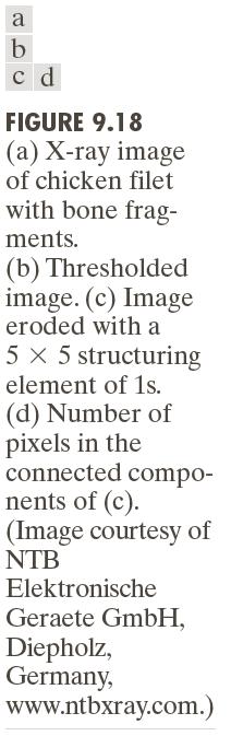
66 For any wavelength of light in the visible spectrum, the tristimulus values needed to produce the color coresponding to that wavelength can be obtained from the existing curves or tables. Another approach for specifying colors is to use the CIE chromaticity diagram, which shows color compositin as a function of x (red) and y (green); z (blue) is obtained from relation z = 1-x-y.

67 Digital Image Processing

68 The positions of the various spectrum colors (from violet at 380 nm to red at 780 nm) are indicated around the boundary of the tongue-shaped chromaticity diagram. The chromaticity diagram is useful for color mixing because a straight-line segment joining any two points in the diagram defines all the different color variation that can be obtained by combining these two colors. This procedure can be extended to three colors: to triangle determined by the three

69 color-points on the diagram embodies all the possible colors that can be obtained by mixing the three colors.

70 Color Models A color model (color space or color system) is a specification of a coordinate system and a subspace within that system where each color is represented by a single point. Most color models in use today are oriented either toward hardware (color monitors or printers) or toward applications where color manipulation is a goal.

71 The most commonly used hardware-oriented model is RGB (red-green-blue) for color monitors, color video cameras. The CMY (cyan-magenta-yellow) and CMYK (cyan-magenta-yellow-black) models are in use for color printing. The HSI (hue-saturation-intensity) model corespond with the way humans describe and interpret colors. The HSI model has the advantage that it decoupes the color and gray-scale information in an image, making it suitable for using the gray-scale image processing techniques.

72 The RGB Color Model In the RGB model, each color appears decomposed in its primary color components: red, green, blue. This model is based on a Cartesian coordinate system. The color subspace of interest is the unit cube (Figure 6.7), in which the primary and the seconadary colors are at the corners; black is at the origin, and white is at the corner farthest from the origin.

73 The gray scale (point of equal RGB values) extends from black to white along the line joining these two points. The different colors in this model are points on or inside the cube, and are defined by vectors extending from the origin.

74 Images represented in the RGB color model consist of three component images, one for each primary color. The number of bits used to represent each pixel in RGB space is called the pixel depth. Consider an RGB image in which each of the red, green, and blue images are an 8-bit image. In this case, each

75 RGB color pixel has a depth of 24 bits. The term full-color image is used often to denote a 24-bit RGB color image. The total number of colors in a 24-bit RGB image is A convenient way to view these colors is to generate color planes (faces or cross sections of the cube).

76 A color image can be acquired by using three filters, sensitive to red, green, and blue.

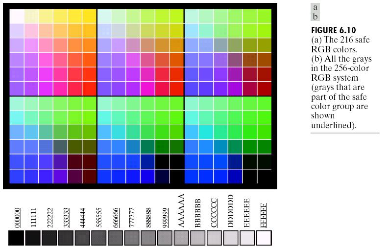
77 Because of the variety of systems in use, it is of considerable interest to have a subset of colors that are likely to be reproduced faithfully, resonably independently of viewer hardware capabilities. This subset of colors is called the set of safe RGB colors, or the set of all-systems-safe colors. In Internet applications, they are called safe Web colors or safe browser colors. We assume that 256 colors is the minimum number of colors that can be reproduced faithfully by any system. Forty of

78 these 256 colors are known to be processed differently by varoius operating system. We have 216 colors that are common to most systems, and are the safe colors, especially in Internet applications. Each of the 216 safe colors has a RGB representation with: RG,, B 0,51,102,153, 204, 255 We have (6) 3 =216 possible color values. It is costumary to express these values in the hexagonal number system.

79 Each safe color is formed from three of the two digit hex numbers from the above table. For example purest red if FF0000. The values and FFFFFF represent black and white respectively. Figure 6.10(a) shows the 216 safe colors, organized in descending RGB values. Figure 6.10(b) shows the hex codes for all the possible gray colors in the 216 safe color system. Figure 6.11 shows the RGB safe-color cube.

80

81 The CMY and CMYK Color Models Cyan, magenta, and yellow are the secondary colors of light but the primary color of pigments. For example, when a surface coated with yellow pigment is illuminated with white light, no blue light is reflected from the surface. Yellow substracts blue light from reflected white light (which is composed of equal amounts of red, green, and blue light). Most devices that deposit color pigments on paper, such as color printers and copiers, require CMY data input and

82 perform RGB to CMY conversion. Assuming that the color values were normalized to range [0,1], this conversion is: C 1 R M 1 G Y 1 B From this equation we can easily deduce, that pure cyan does not reflect red, pure magenta does not reflect green, and pure yellow does not reflect blue.

83 Equal amount of pigments primary, cyan, magenta, and yellow should produce black. In practice, combining these colors for printing produces a muddy-looking black. In order to produce true black (which is the predominant color in printing), a fourth color, black, is added, giving rise to the CMYK color model.

84

85 The HSI Color Model The RGB, CMY, and other similar color models are not well suited for describing colors in terms that are practical for human interpretation. We (humans) describe a color by its hue, saturation and brightness. Hue is a color attribute that describes a pure color, saturation gives a measure of the degree to which a pure color is diluted by white light and brightness is a subjective descriptor that embodies the achromatic notion of intensity.

86 The HSI (hue, saturation, intensity) color model, decouples the intensity component from the color information (hue and saturation) in a color image. What is the link between the RGB color model and HSI color model? Consider again the RGB unit cube. The intensity axis is the line joining the black and the white vertices. Consider a color point in the RGB cube. Let P be a plane perpedicular to the intensity axis and containing the color point. The intersection of this plane with the intensity axis gives us the

87 intensity of the color point. The saturation (purity) of the considered color point increases as a function of distance from the intensity axis (the saturation of the point on the intensity axis is zero). In order to determine how hue can be linked to a given RGB point, consider a plane defined by black, white and cyan. The intensity axis is also included in this plane. The intersection of this plane with the RGB-cube is a triangle. All point contained in this triangle would have the same hue (i.e. cyan).

88 The HSI space is represented by a vertical intensity axis and the locus of color points that lie on planes perpedicular to this axis. As the planes move up and down the intensity axis, the boundary defined by the intersection of this plane with the faces of the cube have either triangular or hexagonal shape.

89

90 In the plane shown in Figure 6.13(a) primary colors are separated by 120º. The secondary colors are 60º from the primaries. The hue of the point is determined by an angle from some reference point. Usually (but not always) an angle of 0º from the red axis designates 0 hue, and the hue increases countercloclwise from there. The saturation (distance from the vertical axis) is the length of the vector from the origin to the point. The origin is defined by the intersection of the color plane with the vertical intensity axis.

91 Converting colors from RGB to HSI if B G H 360 if B G ( RG) ( RB) arccos 2 2 ( RG) ( RB)( GB) 3 S 1 min{ R, G, B} R G B 1 I RG B 3

92 It is assumed that the RGB values have been normalized to the range [0,1] and that angle θ is measured with respect to the red axis of the HSI space in Figure Hue can be normalized to the range [0,1] by dividing it to 360º. The other two HSI components are in this range if the RGB values are in the interval [0,1]. R=100, G=150, B=200 H=210º, S=1/3, I=150/255=0.588

93 Converting colors from HSI to RGB Given values of HSI we now want to find the corresponding RGB values in the same range. RG sector (0º H < 120º) B I(1 S) Scos H R I1 cos(60 H ) G 3 I ( R B)

94 GB sector (120º H < 240º) R I(1 S) Scos H H H 120, G I 1 cos(60 H ) B 3 I ( RG) BR sector (120º H < 240º) G I(1 S) Scos H H H 240, B I 1 cos(60 H ) R 3 I ( GB)

95 Pseudocolor Image Processing Pseudocolor (also called false color) image processing consists of assigning colors to gray values based on a specified criterion. The main use of pseudocolor is for human visualization and interpretation of gray-scale events in an image or sequence of images.

96 Intensity (Density) Slicing If an image is viewed as a 3-D function, the method can be described as one of placing planes parallel to the coordinate plane of the image; each plane then slices the function in the area of intersection.

97 The plane at f( x, y) li slices the image function into two levels. If a different color is assigned to each side of the plane, any pixel whose intensity level is above the plane will be coded with one color and any pixel below the plane will be coded with other color. Levels that lie on the plane itself may be arbitrarily assigned one of the two colors. The result is a two color image whose relative appearance can be controlled by moving the slicing plane up and down the intensity axis.

98 Let [0, L-1] represent the gray scale, let l0 represent black (f(x,y)=0) and level ll-1 represent white (f(x,y)=l-1). Suppose that P planes perpendicular to the intensity axis are defined at levels l1, l2,, lp, 0<P<L-1. The P planes partition the gray scale into P+1 intervals, V1, V2,, VP+1. Intensity to color assignments are made according to the relation: f( x, y) c if f( x, y) V. k k

99 Measurements of rainfall levels with ground-based sensors are difficult and expensive, and total rainfall figures are even more difficult to obtain because a significant portion of

100 precipitations occurs over the ocean. One way to obtain these figures is to use a satellite. The TRMM (Tropical Rainfall Measuring Mission) satellite utilizes, among others, three sensors specially designed to detect rain: a precipitation radar, a microwave imager, and a visible and infrared scanner. The results from the various rain sensors are processed, resulting in estimates of average rainfall over a given time period in the area monitored by the sensors. From these estimates, it is not difficult to generate gray-scale images whose intensity values

101 correspond directly to rainfall, with each pixel representing a physical land area whose size depends on the resolution of the sensors.

102 Basics of Full-Color Image Processing cr( x, y) R( x, y) 3 4 f : D /, f( x, y) c cg ( x, y) G( x, y) cb ( x, y) B( x, y) C( x, y) M( x, y) f( x, y) c Y( x, y) K( x, y)

103 Color Transformations - processing the components of a color image within the context of a single-color model i i 1 2 n gxy (, ) T f( xy, ) s T( r, r,..., r ), i 1,2,..., n ( f( x, y) r, g( x, y) s) ri, si are the color components of f(x, y) and g(x, y), n is the number of color components, and {T1, T2,, Tn} is a set of transformations or color mapping functions that operate on ri to produce si. (n=3 or n=4)

104

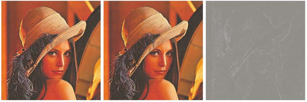
105 In theory, any transformation can be performed in any color model. In practice, some operations are better suited to specific color models. Suppose we wish to modify the intensity of a color image, using gxy (, ) kf( xy, ), 0 k 1 In the HSI color space, this can be done with: s1= r1, s2= r2, s3=k r3

106 In the RGB/CMY color model all components must be transformed s1= kr1, s2= kr2, s3=kr3 (RGB) si = kri+(1-k), i=1,2,3 (CMY) Although the HSI transformation involves the fewest number of operations, the costs for converting an RGB or CMY(K) image to the HSI color space are much bigger than the transformations.

107

108 Color Complements The hues directly opposite one another on the above color circle are called complements (analogous to the gray-scale negatives).

109

110 Unlike the intensity transformation, the RGB complement transformation functions used in this example do not have straightforward HSI space equivalent. The saturation component of the complement cannot be computed from the saturation component of the input image alone. Color Slicing Highlighting a specific range of colors in an image is useful for separating objects from their surroundings. The basic idea is either to:

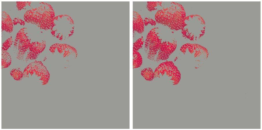
111 - display the colors of interest so they stand out from the background - use the region defined by the colors as a mask for further processing. One of the simplest ways to slice a color image is to map the colors outside some range of interest to a neutral color. If the colors of interest are enclosed by a cube (or hypercube, if n>3) of width W and centered at a

112 prototypical (e.g. average) color with components a1, a2,..., a n the set of transformations is: W 0.5 if rj aj, 1 j n si 2, i 1,2,..., n ri otherwise These transformations highlight the colors around the prototype by forcing all other colors to the midpoint of the reference color space (an arbitrarily chosen neutral point).

113 For the RGB color space, for example, a suitable neutral point is middle gray or color (0.5, 0.5, 0.5). If a sphere is used to specify the colors of interest, the transformations are: n if ( rj aj) R0 si j1, i 1,2,..., n ri otherwise where R0 is the radius of the enclosing sphere and a1, a2,..., a n are the components of its center.

114

115 Tone and Color Corrections The effectiveness of such transformations is judged ultimately in print. The transformations are developed and evaluated on monitors. It is necessary to have a high degree of consistency between the monitors and the output devices. This is best accomplished with a device-independent color model that relates the color gamut of the monitors and output devices, as well as any other devices being used, to one another. The model of choice for many color management systems (CMS)

116 is the CIE L*a*b* model, also called CIELAB. The L*a*b* color components are given by the following equations: Y L* 116h 16 Y W X Y a* 500h h XW YW Y Z b* 200h h YW ZW

117 3 q q hq ( ) q q XW, YW, Z W are reference tristimulus values typically the white of a perfectly reflecting diffuser under CIE standard D65 illumination ( x , y , z 1 x y). The L*a*b* color space is colorimetric (i.e. colors perceived as matching are encoded identically), perceptually uniform (i.e. color differences among various hues are perceived

118 uniformly), and device independent. Like the HSI system, the L*a*b* system is an excellent decoupler of intensity (represented by lightness L*) and color (represented by a* for red minus green and b* for green minus blue), making it useful in both image manipulation (tone and contrast editing) and image compression applications.

119 Histogram Processing It is not advisable to histogram equalize the components of a color image independently. This can produce wrong colors. A more logical approach is to spread the color intensity uniformly, leaving the colors (e.g., hues) unchanged. The HSI color space is ideally suited for this type of approach.

120 The unprocessed image contains a large number of dark colors that reduce the median intensity to Histogram equalizing the intensity component, without altering the hue and saturation produced image Figure 6.37(c). The image is brighter. Figure 6.37(d) was obtained by increasing also the saturation component.

121 Color Image Smoothing Let Sxy denote a neighborhood centered at (x,y) in an RGB color image. The average of the RGB component vectors in this neighborhood is: 1 c( x, y) c( s, t) K ( st, ) S xy 1 Rst (, ) K ( st, ) Sxy 1 c( x, y) G( s, t) K ( st, ) Sxy 1 Bst (, ) K ( st, ) Sxy

122

123

124 Color Image Sharpening gxy f xy c f xy 2 (, ) (, ) (, ) 2 Rxy (, ) cxy (, ) Gxy (, ) 2 Bxy (, ) 2 2

125

126 Other color spaces YIQ for the NTSC (National Television System Committee) television system in US Y luminance I (in-phase), Q (quadrature) chrominance YUV for the PAL (Phase Alternation Line) and SECAM (Séquentiel Couleur à Mémoire) television system in Europe (I, Q) obtained by rotating (U,V) YCbCr digital video transmission More about color spaces in: Andreas Koschan, Mongi Abidi, Digital Color Image Processing, Wiley, 2008

127 Color Difference RGB, CMY, Lab Euclidean distance HSI - F1=(H1, S1, I1), F2=(H2, S2, I2) d ( F, F ) ( I) ( C), I I I HSI C S S 2S S cos H1 H2 if H1 H2 2 H1 H2 if H1 H2