Part I: Theoretical Background and Integration-Based Methods

Transcription

1 Large Vector Field Visualization: Theory and Practice Part I: Theoretical Background and Integration-Based Methods Christoph Garth

2 Overview Foundations Time-Varying Vector Fields Numerical Integration Geometric Methods Integral Curves Integral Surfaces Advanced Geometric Methods

3 Motivation Point of departure: Vector fields are integral constituents in many scientific application domains Astrophysics, Fusion, Medicine, Fluid Flow,... Flow & vector field visualization is an ingredient in answering typical science questions How & why are things transported? Where do things end up? How do things mix?

4 Mathematical Framework So... what is a vector field? Simple answer: a map v : I D IR n I IR, D IR n that returns a direction and speed for every point in a domain.

5 Vector Fields Simplest way to visualize vector fields: draw arrows or glyphs.

6 Vector Fields Simplest way to visualize vector fields: draw arrows or glyphs.

7 Vector Fields Simplest way to visualize vector fields: draw arrows or glyphs. Glyphs do not describe and provide insight into transport or mixing...

8 Vector Fields Vector fields induce a family of ordinary differential equations (ODEs): dx dt = v(t, x) x(t 0 )=x 0 ODE initial condition (x 0,t 0 ) Any solution for a given is called integral curve, trajectory or orbit.

9 Vector Fields Graphically: v v (t 0,x 0 ) v

10 Vector Fields Drawing trajectories is a simple way to visualize vector fields and convey some insight. Intuition: idealized particles, embedded in a flow. Thermal Mixing, P. Fischer, ARNL

11 Vector Fields Drawing trajectories is a simple way to visualize vector fields and Integral convey curves some provide insight. a simple answer to two basic (but important!) questions: Intuition: idealized particles, embedded in a flow. Where do things go? Where are things coming from? Modern analysis of transport and mixing is based on study of integral curves (more later). Thermal Mixing, P. Fischer, ARNL

12 Numerical Integration Closed form solutions (analytic) to integral curve ODE are not available in general Numerical approximation / ODE solvers ODE solvers come in many shapes and sizes vector field properties approximation properties,... numerical properties

13 Numerical Integration Euler method: simplest method, fast, inaccurate, unstable x n+1 = x n + t v(x n,t n ) (x 4,t 4 ) (x 0,t 0 ) (x 3,t 3 ) (x 1,t 1 ) Error per step (local error): (x 2,t 2 ) O( t 2 )

14 Numerical Integration Heun s method: use Euler as trial step, then improve k1 = v(x n,t n ) k2 = v(x n + t k 1,t n + t) x n+1 = x n + t 2 ( k 1 + k 2 ) Local error: Two stages O( t 3 ) k1 (x 0,t 0 ) k2 (x 1,t 1 )

15 Numerical Integration k1 = v(x n,t n ) k2 = v(x n + t k 1,t n + t) x n+1 = x n + t 2 ( k 1 + k 2 ) can also be written as a table: k1 (x 0,t 0 ) k2 (x 1,t 1 ) ½ ½ Butcher tableau

16 Numerical Integration General: Runge-Kutta schemes Textbook on Numerical ODEs 0 1/2 1/2 1/2 0 1/ /6 1/3 1/3 1/6 k1 = v(x n,t n ) k2 = v(x n + t 2 k 1,t n + t 2 ) k3 = v(x n + t 2 k 2,t n + t 2 ) k4 = v(x n + t k 3,t n + t ) x n+1 = x n ( k 1 +2 k 2 +2 k 3 + k 4 )

17 Numerical Integration General: Runge-Kutta schemes Textbook on Numerical ODEs 0 1/2 1/2 1/2 0 1/ /6 1/3 1/3 1/6 k1 = v(x n,t n ) k2 = v(x n + t 2 k 1,t n + t 2 ) k3 = v(x n + t 2 k 2,t n + t 2 ) k4 = v(x n + t k 3,t n + t ) x n+1 = x n ( k 1 +2 k 2 +2 k 3 + k 4 )

18 Numerical Integration General: Runge-Kutta schemes Textbook on Numerical ODEs 0 1/2 1/2 1/2 0 1/ /6 1/3 1/3 1/6 k1 = v(x n,t n ) k2 = v(x n + t 2 k 1,t n + t 2 ) k3 = v(x n + t 2 k 2,t n + t 2 ) k4 = v(x n + t k 3,t n + t ) x n+1 = x n ( k 1 +2 k 2 +2 k 3 + k 4 )

19 Numerical Integration General: Runge-Kutta schemes Textbook on Numerical ODEs 0 1/2 1/2 1/2 0 1/ /6 1/3 1/3 1/6 k1 = v(x n,t n ) k2 = v(x n + t 2 k 1,t n + t 2 ) k3 = v(x n + t 2 k 2,t n + t 2 ) k4 = v(x n + t k 3,t n + t ) x n+1 = x n ( k 1 +2 k 2 +2 k 3 + k 4 ) 4th-order Runge-Kutta method

20 Numerical Integration General: Runge-Kutta schemes Textbook on Numerical ODEs 0 1/2 1/2 1/2 0 1/ /6 1/3 1/3 1/6 k1 = v(x n,t n ) k2 = v(x n + t 2 k 1,t n + t 2 ) k3 = v(x n + t 2 k 2,t n + t 2 ) k4 = v(x n + t k 3,t n + t ) x n+1 = x n ( k 1 +2 k 2 +2 k 3 + k 4 )

21 Numerical Integration General: Runge-Kutta schemes Textbook on Numerical ODEs 0 1/2 1/2 1/2 0 1/ /6 1/3 1/3 1/6 k1 = v(x n,t n ) k2 = v(x n + t 2 k 1,t n + t 2 ) k3 = v(x n + t 2 k 2,t n + t 2 ) k4 = v(x n + t k 3,t n + t ) x n+1 = x n ( k 1 +2 k 2 +2 k 3 + k 4 )

22 Numerical Integration General: Runge-Kutta schemes Textbook on Numerical ODEs 0 1/2 1/2 1/2 0 1/ /6 1/3 1/3 1/6 k1 = v(x n,t n ) k2 = v(x n + t 2 k 1,t n + t 2 ) k3 = v(x n + t 2 k 2,t n + t 2 ) k4 = v(x n + t k 3,t n + t ) x n+1 = x n ( k 1 +2 k 2 +2 k 3 + k 4 ) 4th-order Runge-Kutta method, 4 stages Local error O( t 5 ), accumulated (global) error: O( t 4 )

23 Numerical Integration Choosing an integration scheme: tradeoff between stages/complexity and accuracy. Higher-order methods are usually more efficient: require less evaluations of v to obtain the same solution accuracy. t How to choose t? In principle, need to make sure that no information is missed smallest possible t for entire dataset?

24 Numerical Integration Adaptive stepsize control, chooses t based on observed vector field complexity. Popular schemes: Runge-Kutta-Fehlberg (RKF / RK45)

25 Numerical Integration Adaptive stepsize control, chooses t based on observed vector field complexity. Popular schemes: Runge-Kutta-Fehlberg (RKF / RK45)

26 Numerical Integration Adaptive stepsize control, chooses t based on observed vector field complexity. Popular schemes: Runge-Kutta-Fehlberg (RKF / RK45) O( t 6 ) O( t 5 )

27 Numerical Integration t Adaptive stepsize control, chooses based on observed vector field complexity. Popular schemes: Runge-Kutta-Fehlberg (RKF / RK45) Six stage provide both order 4 and order 5 approximations Comparing these allows error estimate, increase or decrease in step size in response Many visualization systems (e.g., VTK) implement RKF. Other variants: Cash-Karp (RKCK), Dormand-Prince (DOPRI5)

28 Vector Field Interpolation Numerical integrators treat as a black box: put in position and time, get vector back. x v t But, vector fields are typically given in discrete form over some computational mesh, with vectors associated to points.

29 Vector Field Interpolation Interpolation can be used to reconstruct a continuous mesh from the discrete data: linear interpolation over triangles or tetrahedra trilinear interpolation over hexahedra or voxels non-linear interpolation for other mesh/cell types Hard problem for irregular meshes: which cell contains? x

30 Vector Field Interpolation Typical use case for spatial data structures: octree, kd-tree,... But, modern simulation meshes are complex: Many points and cells (1M 1B) Unstructured, adaptive resolution cells are smaller where vector field more complex strong variation in cell size (factor 1M is not unusual) Non-linear cell types (hex, pyramids, prisms) Holes and complex boundaries

31 Numerical Integration Integration efficiency depends on lookups of : Fast spatial data structure for mesh types that require it v Shameless plug: Fast, Memory-Efficient Cell Location in Unstructured Grids for Visualization, C. Garth, K. I. Joy, Vis 2010 Fast Volume Rendering session, Thursday Reduce the number of lookups, i.e. integration steps? Adaptive stepsize control is key to efficiency!

32 Numerical Integration One more caveat: Visualization requires graphical output... so be constrained to guarantee truthful output: t must? More steps, less efficiency...?

33 Numerical Integration Numerical integration scheme with dense output: Compute a polynomial description of the curve in between the solution points x n Faithful graphical output: sample polynomial in between the x n Dormand-Prince (DOPRI5) 5th-order, six stage, adaptive dense RK scheme

34 Numerical Integration Numerical integration scheme with dense output: Compute a polynomial description of the curve in between the solution points x n Faithful graphical output: sample polynomial in between the x n Dormand-Prince (DOPRI5) 5th-order, six stage, adaptive dense RK scheme

35 Streamlines and Pathlines Direct Integral Curve Visualization Streamlines ( v is constant in time) Pathlines ( varies with time) v

36 Streamlines and Pathlines Other variants: streamribbons, streamtubes Tubes Ribbons

37 Streamlines and Pathlines Animated Particles (also convey speed)

38 Streamlines and Pathlines Streamline is the line traced by a given particle. t0 Streamline is actually a projection along the time axis all particle positions over time are visible simultaneously

39 Streamlines and Pathlines Streamline is the line traced by a given particle. t0 t1 Streamline is actually a projection along the time axis all particle positions over time are visible simultaneously

40 Streamlines and Pathlines Streamline is the line traced by a given particle. t1 t2 t0 Streamline is actually a projection along the time axis all particle positions over time are visible simultaneously

41 Streamlines and Pathlines Streamline is the line traced by a given particle. t0 t1 t2 t3 Streamline is actually a projection along the time axis all particle positions over time are visible simultaneously

42 Streamlines and Pathlines Streamline is the line traced by a given particle. t0 t1 t2 t3 t4 Streamline is actually a projection along the time axis all particle positions over time are visible simultaneously

43 Streamlines and Pathlines Streamline is the line traced by a given particle. t0 t1 t2 t3 t4 t5 Streamline is actually a projection along the time axis all particle positions over time are visible simultaneously

44 Time Lines A time line is a line traced formed by a set of particles. t0 Time lines do not show trajectories rather, they capture the line of particles at a given instant in time.

45 Time Lines A time line is a line traced formed by a set of particles. t1 Time lines do not show trajectories rather, they capture the line of particles at a given instant in time.

46 Time Lines A time line is a line traced formed by a set of particles. t2 Time lines do not show trajectories rather, they capture the line of particles at a given instant in time.

47 Time Lines A time line is a line traced formed by a set of particles. t3 Time lines do not show trajectories rather, they capture the line of particles at a given instant in time.

48 Time Lines A time line is a line traced formed by a set of particles. t4 Time lines do not show trajectories rather, they capture the line of particles at a given instant in time.

49 Time Lines A time line is a line traced formed by a set of particles. t5 Time lines do not show trajectories rather, they capture the line of particles at a given instant in time.

50 Streak Lines A streak line is a line of particles that are released incrementally into the flow. t0 0 Streak lines do not show trajectories rather, they capture the line of particles at a given instant in time.

51 Streak Lines A streak line is a line of particles that are released incrementally into the flow. t1 0 1 Streak lines do not show trajectories rather, they capture the line of particles at a given instant in time.

52 Streak Lines A streak line is a line of particles that are released incrementally into the flow. t Streak lines do not show trajectories rather, they capture the line of particles at a given instant in time.

53 Streak Lines A streak line is a line of particles that are released incrementally into the flow. t Streak lines do not show trajectories rather, they capture the line of particles at a given instant in time.

54 Streak Lines A streak line is a line of particles that are released incrementally into the flow. t Streak lines do not show trajectories rather, they capture the line of particles at a given instant in time.

55 Streak Lines A streak line is a line of particles that are released incrementally into the flow. t Streak lines do not show trajectories rather, they capture the line of particles at a given instant in time.

56 Integral Curve Comparison

57 Integral Curve Comparison Physical Experiment Délery, 2005

58 Time-Varying Datasets Small data: regular mesh 12 bytes/vector (3x float) = 24 MB x 500 timesteps = 11.7 GB total Interpolation is usually done linearly/cubically between time slices. Can t afford a random-access policy. Arrange algorithm such that data can be streamed, i.e. time slices are read once and discarded after use.

59 Integral Curves Direct visualization of integral curves: limited visual scalability

60 Integral Surfaces Integral surface: surface spanned by a family of integral curves

61 Integral Surfaces Integral surface: surface spanned by a family of integral curves

62 Integral Surfaces Integral surface: surface spanned by a family of integral curves

63 Integral Surfaces Integral surface: surface spanned by a family of integral curves

64 Integral Surfaces Integral surface: surface spanned by a family of integral curves

65 Integral Surfaces Example: seeding curve

66 Integral Surfaces Streaming Stream & Path Surface Construction Garth, Krishnan, Bobach, Hagen, Joy, Vis 2008 Integral surface approximation is performed in two phases: Phase 1: Time line approximation (streaming) Phase 2: Triangulation

67 Phase 1: Time Line Approximation Integral Surfaces are a set of integral curves. a set of time lines, or t1 t2 t3 t4 t0 Approximation Algorithm: Approximate surface by a finite set of time lines (skeleton) Discretize time lines using a finite set of integral curves Approximate time line ti+1 from time line ti t0

68 Phase 1: Time Line Approximation Step 1: Compute initial approximation, points on t1 are advected from t0 t1 t0

69 Phase 1: Time Line Approximation Step 1: Compute initial approximation, points on t1 are advected from t0 t1 t0

70 Phase 1: Time Line Approximation Step 2: Apply refinement predicate on adjacent point triples to determine where better resolution is needed t1 t0

71 Phase 1: Time Line Approximation Step 2: Apply refinement predicate on adjacent point triples to determine where better resolution is needed t1 t0

72 Phase 1: Time Line Approximation Step 2: Apply refinement predicate on adjacent point triples to determine where better resolution is needed t1 t0

73 Phase 1: Time Line Approximation Step 2: Apply refinement predicate on adjacent point triples to determine where better resolution is needed t1 t0

74 Phase 1: Time Line Approximation Step 3: Insert new points next to the insufficient points t1 t0

75 Phase 1: Time Line Approximation Step 3: Insert new points next to the insufficient points t1 t0

76 Phase 1: Time Line Approximation Repeat at Steps 2 and 3 until no further refinement is needed t1 t0

77 Phase 1: Time Line Approximation Approximate sequence of timelines going from ti to ti+1 t2 t1 t0

78 Phase 1: Time Line Approximation Approximate sequence of timelines going from ti to ti+1 t1 t2 t3 t0

79 Phase 1: Time Line Approximation Approximate sequence of timelines going from ti to ti+1 t2 t3 t1 t4 t0

80 Phase 1: Time Line Approximation Result: Surface skeleton of integral curves + time lines t2 t3 t1 t4 t0

81 Refinement Predicates Predicates: Thresholds on local curve properties such as derivative and curvature. δ point distance γ A triangle area inter-point angle

82 Phase 2: Surface Triangulation Discretize integral curves to obtain a point set on the surface. t2 t3 t1 t4 t0

83 Phase 2: Surface Triangulation Discretize integral curves to obtain a point set on the surface. t2 t3 t1 t4 t0

84 Phase 2: Surface Triangulation Use adjacent integral curves ( strip) and triangulate heuristically. t2 t3 t1 t4 t0

85 Phase 2: Surface Triangulation Use adjacent integral curves ( strip) and triangulate heuristically. Shortest diagonal advancing front works well t2 t3 t1 t4 t0

86 Phase 2: Surface Triangulation Use adjacent integral curves ( strip) and triangulate heuristically. Shortest diagonal advancing front works well t2 t3 t1 t4 t0

87 Phase 2: Surface Triangulation Use adjacent integral curves ( strip) and triangulate heuristically. Shortest diagonal advancing front works well t2 t3 t1 t4 t0

88 Phase 2: Surface Triangulation Use adjacent integral curves ( strip) and triangulate heuristically. Shortest diagonal advancing front works well t2 t3 t1 t4 t0

89 Phase 2: Surface Triangulation Use adjacent integral curves ( strip) and triangulate heuristically. Shortest diagonal advancing front works well t2 t3 t1 t4 t0

90 Phase 2: Surface Triangulation Use adjacent integral curves ( strip) and triangulate heuristically. Shortest diagonal advancing front works well t2 t3 t1 t4 t0

91 Phase 2: Surface Triangulation Use adjacent integral curves ( strip) and triangulate heuristically. After an insertion point, triangulated recursively t2 t3 t1 t4 t0

92 Phase 2: Surface Triangulation Use adjacent integral curves ( strip) and triangulate heuristically. After an insertion point, triangulated recursively t2 t3 t1 t4 t0

93 Phase 2: Surface Triangulation Use adjacent integral curves ( strip) and triangulate heuristically. After an insertion point, triangulated recursively t2 t3 t1 t4 t0

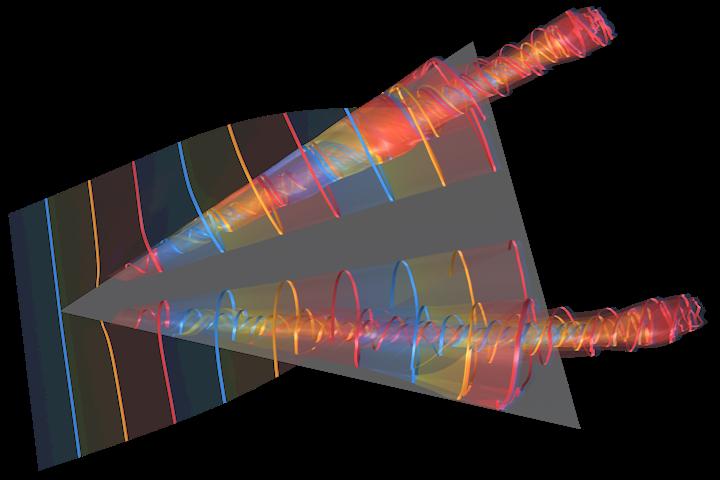
94 Experiments Delta wing dataset (18M cells, 1000 timesteps)

95 Examples Delta wing dataset (18M cells, 1000 timesteps)

96 Examples Delta wing dataset (18M cells, 1000 timesteps)

97 Examples

98 Examples

99 Examples

100 Examples

101 Visualization Example: Car (stationary, 27M cells)

102 Visualization Example: Car (stationary, 27M cells)

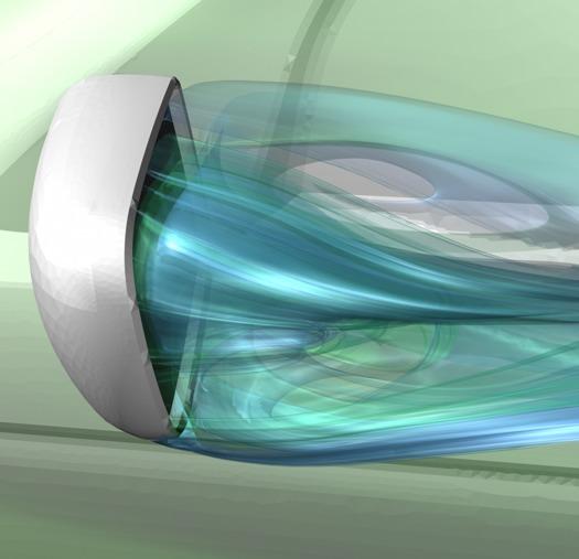
103 Visualization Example: Car (stationary, 27M cells)

104 Time and Streak Surfaces Krishnan, Garth, Joy, Vis 2009: Similar approach for time and streak surfaces using triangle meshes Mesh adaptation through splits collapses flips

105 Time and Streak Surfaces Krishnan, Garth, Joy, Vis 2009: Similar approach for time and streak surfaces using triangle meshes Mesh adaptation through splits collapses flips

106 Streak Surfaces 95

107 Krishnan, Garth, Joy, 2009: Similar approach for time and streak surfaces using triangle meshes 96

108 Krishnan, Garth, Joy, 2009: Similar approach for time and streak surfaces using triangle meshes 96

109 Time and Streak Surfaces

110 Time and Streak Surfaces

111 Time and Streak Surfaces Approximate method: Smoke Surfaces [von Funck et al., Vis 2008] Start with high-res time or streak surface, no adaptation As the triangulation degenerates, smoothly fade it out Transparency term is physically inspired, mimics appearance of smoke [von Funck et al., Vis 2008]

112 Time and Streak Surfaces Approximate method: Smoke Surfaces [von Funck et al., Vis 2008] Start with high-res time or streak surface, no adaptation As the triangulation degenerates, smoothly fade it out Transparency term is physically inspired, mimics appearance of smoke [von Funck et al., Vis 2008]

113 References Additional references at tutorial/materials.html

114 Questions?