Generating a New Shapefile

Transcription

1 Week 9

2 Generating a New Shapefile STEPS 1) Select a appropriate folder or folder connection in the Catalog tree. 2) Click on Contents tab and move cursor into that window 3) Right click in that window and select. New toggle in the popup list to: Shapefile 4) Click in the Name text box and type a name for the new shapefile. 5) Click the Feature Type drop-down arrow and click the type of geometry the shapefile will contain. 6) Click Edit to define the shapefile's coordinate system. 7) Select, import, or define a new coordinate system. It's highly recommended that you define the shapefile's coordinate system now; however, you can postpone this step until a later time. 8) Click OK. 9) If the shapefile will store polylines representing routes, check Coordinates will contain M values. 10) If the shapefile will store three-dimensional features, check Coordinates will contain Z values. 11) Click OK. The new shapefile appears in the folder's contents.

3 Generating a New Shapefile

4 Generating a New Shapefile

5 Generating a New Shapefile Feature Types: Point Line??? Polygon Polyline Multipoint Multipatch

6 Advanced Feature Types Polyline Polygon POLYLINE Multiple line features stored as a single object No polygon items or attributes Unlike a single line feature, polylines can have multiple thicknesses assigned etc. (e.g., county road, State HWY, US HWY) Used in Dynamic Segmentation Dynamic Seg. Point and Line Events in one Endpoints

7 Advanced Feature Types MULTIPATCH A 3D geometry used to represent the outer surface, or shell, of features that occupy a discrete area or volume in 3D space. Here, planar 3D rings and triangles are used in combination to model a 3D shell. Multipatches used to represent spheres, cubes, & isosurfaces to form complex 3D shapes..e.g., buildings

8 Advanced Feature Types MULTIPOINT Sometimes, you need to create a feature that has more than one physical part but only references one set of attributes in the database. These are called multipoint features. Mass point observations from lidar data are often represented in a feature class with multipoint geometry.

9 Back to the Shapefile Define Coordinates: UTM NAD83, Zone 15 N Then you re ready to open it in ArcGIS for editing

10 GIS Input Methods 1) Key board inputs x, y, attribute etc. 2) Land Survey & COGO Section or ¼ section corners & use COGO to determine within-section parcel lines 3) Scanning & automatic line digitizing (R2V, VTRAC, etc) 4) Heads-Up digitizing directly form digital maps/photos/images Manually digitize info right off the computer screen Avoids some of the problems associated with paper map digitizing. Humidity affects paper map shape/size from day to day errors Resulting digital line-work propagates these error Difficult to reconcile hard to know what is right Scanning freezes the error in time, which remains constant day-to-day 5) Data input can become a major bottleneck of a GIS project Can cost 80% or more of project time Labor intensive, tedious, error-prone Constructing the GIS data can be so large that the project never finishes 6) Digitizing Bottom Line It is worth your while to do it as efficiently as possible

11 Digitizing Tips Use the highest quality images available Maximizes the potential accuracy that may be required for a GIS project 61 cm 1 m 5 m More vertices creates smoother, potentially more accurate representations of reality. Vertex density is often project & scale specific Shoreline digitizing for beach erosion (1:15,840) Land use land cover studies (1:50,000 1:100,000) In general, hyper vertex placement is often an unnecessary waste of time & effort Preserving the character of complex shapes vs. Placing hundreds of vertices along straight lines Try to NOT double digitize Also a waste of time and effort Time to retrace what has already been done Time needed to edit/clean up sliver polygons etc. afterward

12 Heads-Up Digitizing in ArcGIS

13 Heads-Up Digitizing in ArcGIS Arc/INFO used to handle this during performance of BUILD & CLEAN functions with options <snap distance> <weed tolerance> set accordingly ArcGIS has functions that now allow one to completely avoid these problems

14 Heads-Up Digitizing in ArcGIS

15 Cutting Polygons & Island Polygons

16 GPS Forecasting: Trimble s PLANNING 1) Navigate to ftp://ftp.trimble.com/pub/eph/ 2) Open current Almanac 3) Copy it into notepad & save as name.alm 4) Open Planning, import ALM data, and set location or city

17 START HERE

18 Vector vs. Raster GIS Vector-based GIS Discrete data - Discrete either in/on a polygon/line or not no fuzziness in between - Stores graphic information as a series of points or nodes - All connecting lines are straight between nodes - Keeps all X, Y coordinates - Can accurately represent boundaries, but is computationally demanding Raster-based GIS Continuous data (Inherently fuzzy, seldom has clear boundaries) - Stores graphic information as a series of cells with a wide range of possible values - 8-bit integers (0-255 signed or not) Landsat & SPOT - 16-bit integers ( signed or not) AVHRR, MODIS, QuickBird - Single/Double/Quadruple precision floating point (32-bit/64-bit/128-bit) - Ex: DEM data, LIDAR data, weather-climate data - Rapid computation at expense of accuracy Developed Agricultural Forest Water Wetlands Barren Land - Data organized by ROW & COLUMN addressing

19 Discrete vs. Continuous Data Continuous Data Data in which each location on the surface is A relationship from a fixed point in space or From a fixed emitting source or frame of reference Examples: Elevation the fixed point being mean sea level (MSL) Aspect the fixed point being direction (N,S,E,W) Satellite data - the fixed point being orientation w/ref to sun & terrain Forested Lands or tree density blends of species or bole arrangements Discrete Data Object has a known or definable boundaries Easy to define precisely where the object/feature begins and ends Usually nouns: cover type, agricultural field, water bodies, lamp posts Discrete Data Examples: Lake shore, buildings, roads, etc. Aspect the fixed point being direction (N,S,E,W) Forested Lands or tree density blends of species or arrangements

20 Continuous vs. Discrete Raster Data

21 Continuous vs. Discrete Raster Data

22 Continuous vs. Discrete Raster Data

23 Continuous vs. Discrete Raster Data

24 Continuous vs. Discrete Raster Data

25 Continuous vs. Discrete Raster Data Continuous DEM Continuous PALSAR Continuous Landsat (TM) Discrete TM Classification Single precision floating point 16-bit unsigned Integer 8-bit unsigned integer per band (7) 8-bit unsigned integer

26 Rows (Y) Discrete (or Categorical) Raster Data Discrete TM Classification Columns (X)

27 Surface vs. Feature Features are attributes (name, color, size, etc) given to a point, line, or a polygon Surface is a term used in GIS to define a raster layer (DEM, rainfall, etc.) represent phenomena that have values at every point across their extent. And, shows how continuous data can change These values are often derived from a limited set of sample values, either. based on direct measurement Gold/silver ore concentrations from sample locations Surface temperature values from a network of weather reporting stations Or, mathematically derived from other data slope & aspect surfaces derived from an elevation surface surface of distances from bus stops in a city surfaces showing concentration of criminal activity or probability of lightning strikes. In the point sampling case (without ancillary data), values between points are often estimated by interpolation (leans heavily on assumption of spatial autocorrelation) Or, modeled using ancillary data relationships between point data & ancillary data (e.g., satellite data).

28 Surface: Interpolation & Modeling Surfaces are often depict probabilities Probability of an archeological site being near a stream Probability of a bobolink occurrence modeling based on sampling + habitat Probability of deer infection by CWD sample data cause remains a mystery Point-based Interpolation Surface Point-based + ancillary data modeled surface Estimated Ozone Depletion Surface

29 Surface: Spatial Modeling POINT SAMPLING DATA (120 plots) Canopy Diameter Crown Closure DBH Length of Live Crown Tree Height Basal Area ANCILLARY DATA Multi-spectral Satellite data MODEL Linear relationships between point data & reflectance at those points SPATIAL ESTIMATION Apply model to all other pixels locations

30 Problems Best Suited to Raster GIS Data When one is dealing with continuous phenomena with out exact boundaries Ex: Spread of oil pollutants from a point source over time

31 Problems Best Suited to Raster GIS Data continuous phenomena with out exact boundaries. Spread of air-borne pollutants from a point source over time

32 Surface Analysis Surfaces can be represented using contour or iso-lines arrays of points TINs Rasters However, most surface analysis in GIS is done on raster or TIN data. Contours are sets of lines of equal value across a surface. Points can be regularly or irregularly distributed across a surface. They are usually used as input to interpolation, kriging, or triangulation tools TINs are nets of triangular facets defined by nodes and edges that cover a surface.

33 Contouring Min 185m, Max 690m, Interval 25m

34 Interpolation Methods Inverse Distance Weighting (IDW) Determines missing values via a linearly weighted combination of sample points N (Arc s Default N = 12). Closer sample point neighbors are given greater weight. Interpolated surface should be that of a locationally dependent variable values depend on spatial location elevation, surface temperature etc. Where u(x) = interpolated value, u, at some point, x, based on i = 0,,N samples u i = u(x i ) the distance weight function w i (x) Where p is the power parameter

35 Interpolation Methods Splines (Bspline, Bezier, Cubic, ) Estimates grid cell values by fitting a minimum-curvature surface to the sample data. Like a flexible sheet of plastic that passes through each data point. But, bends as little as possible TENSION option is more ridged and considered more realistic than the REGULARIZED (integrated average) option in ArcGIS. Cubic spline is common due to smoothness of curve pieces (between 2 points) The spline function for each piece is defined as S i = a i + b i (x x i ) + c i (x x i ) 2 With coeficients a i b i c i to be determined by solving the governing continuity on each spline boundary which involves approximating the first derivative of each piece between points x and x i

36 Interpolation Methods Natural Neighbors based on Voronoi tessellations Surface created using a neighbor technique via a weighted average of sample points. Surface will not exceed MIN or MAX of sample data Voronoi tessellations (Euclidean distances) Colored circles represent interpolating weights w i that are calculated based on the ratio of the shaded area to that of the cell area of the surrounding points. n Basic 2D equation is: G x, y = i=1 w i f(x i, y i ) Where: G x, y is the estimate at (x i, y i ) And: f(x i, y i ) are the known data at (x i, y i )

37 Interpolation Methods Kriging (uses spatial autocorrelation) Sort of like IDW, but Kriging is more sophisticated A = range a Semi-Variograms c o + c Centered around the idea that point sample that are closer in space tend to be more correlated that distant points. (Gold Mining) c o c Interpolates surfaces based on weights inferred from the spatial structure of the input data (via a SEMI-VARIOGRAM) Things that are closer in space tend to be more correlated SPATIAL AUTOCORRELATION Spherical Circular Gaussian Exponential Semivariogram(distance h) = 0.5 * average [ (value at location I value at location j) 2 ]

38 Semi-variogram parameters some Lag distance h} = 0.5 * average [ (value at location X value at location [X i + h]) 2 ] Lag (h) = the distance between pair of sample points being measured. For example, in remote sensing this would be h=1 1 pixel separation h=2 2 pixel separation h=43 43 pixel separation. c o a c o + c c a = the range parameter, and is the distance limit of spatial autocorrelation That is, points farther than this distance are not correlated at all. Co = the nugget parameter, and is variability between spatially close points that is not related to distance. Is either error in measurement or some other variability.originally corresponded to presence of gold deposits hence, nugget. Co + C = the sill parameter, and is equivalent to the over all variance in you data points. C = Distance from the nugget to the SILL

39 Modeled Semivariance

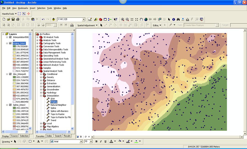
40 Exercise Min = 183 m Max = 690 m 500 sample points

41 Exercise Modeled Semivariogram of the 500 sample points (Gaussian Model) Range (a) = 14.67km Sill (C + Co) variance = 32,300 (or a Standard Deviation of m) Nugget (Co) = 600 m

42 Exercise

43 Exercise

44 Exercise

45 Exercise