GIS Tools - Geometry. A GIS stores data as different layers of information Different feature types are stored in individual files.

Transcription

1

2 A Definition of GIS GIS is a system of hardware, software, and procedures designed to support the capture, management, manipulation, analysis, modeling and display of spatially referenced data for solving complex planning and management problems

3 A GIS stores data as different layers of information Different feature types are stored in individual files Vector models GIS Tools - Geometry Polygons (lakes) Lines (rivers) Points (water wells) Raster models Pixels

4 GIS Tools - Attribute Tables Spatial features are not static GIS layers are linked to database tables, also referred to as attribute tables

5 Attribute Data and Databases Type Name Species 01 Point Birch 02 Point Oak Type Object Length 01 Polyline Stream Polyline Pathway 3 Type Object Area 01 Polygon Clay Soil.4

6 Introduction to Geographic Information Systems D. Spatial Data Files 3) Spatial Data File Formats ( Data Models how data are recorded on the computer) 1. Several formats/models are available 2. Use depends on application 3. Separated into two primary categories a) VECTOR discrete geographic features are represented are built by a collection of points, vertices and arcs (lines). b) RASTER the geographic features across an entire area are represented by a continuous set of pixels or cells. September 11, 2007

7

8 u u u What is Spatial analysis? Heart of GIS which Allows to study real-world processes Uses the existing geographic information and generates new information Important use of the analysis is predicting what will happen after certain time which provides the opportunity to select the best possible alternative

9 Functions of GIS Analysis Presentation of Data Presentation of Pattern of data Where are the forest? What is trend of current road network? What is the trend of population distribution? GIS Analysis and prediction What is the total area of forest? Show me the settlements within 1km from road Show me the Districts with pop. Density > 500/sq.km. Where should I build a new building? Identify the suitable area for locating carpet industries. Assuming that a field will produce the same crop next year as this year; what will happen if there is change in stream flow?

10 Overview ArcGIS Spatial Analyst is an extension to ArcGIS Desktop that provides powerful tools for comprehensive, raster-based spatial modeling and analysis. Using ArcGIS Spatial Analyst, you can derive new information from your existing data, analyze spatial relationships, build spatial models, and perform complex raster operations. With ArcGIS Spatial Analyst tools, you can Find suitable locations. Calculate the accumulated cost of traveling from one point to another. Perform land-use analysis. Predict fire risk. Analyze transportation corridors. Determine pollution levels. Perform crop yield analysis. Determine erosion potential. Perform demographic analysis. Conduct risk assessments. Model and visualize crime patterns.

11 Modeling and Analysis ArcGIS Spatial Analyst is fully integrated with ArcGIS Desktop and provides more than 150 tools and functions that users can access in the same environment as the more than 200 other ArcGIS Desktop tools. This allows users to conduct analysis and modeling tasks via ModelBuilder, scripts, dialog boxes, and the command line without having to change environments between processes. Suitability Modeling Surface Creation Surface Analysis Distance Analysis Statistical Analysis Map Algebra and Overlay

12

13 Suitability modeling A suitability model typically answers the question, Where is the best location? whether it involves finding the best location for a new road or pipeline, a new housing development, a retail store or to install new cell phone antenna. For instance, a commercial developer building a new retail store may take into consideration distance to major highways and any competitors' stores then combine the results with land-use, population density, and consumer spending data to decide on the best location for the store. ArcGIS Spatial Analyst derives new information from the overlay of multiple layers, which can then be used to determine the best location.

14 Site selection requirements In this study we consider the following criteria: 1. Altitude: areas with high altitude are preferred in the allocation of the cellular tower 2. Land use: the cellular tower should not be allocated on residential or parks land uses while it is better to allocate the towers on the industrial and vacant land uses 3. The tower should not be allocated within 200 meters from the city landmark 4. Areas that serve higher population density are preferred for the allocation of towers 5. The towers must be allocated within 250 meters from paved roads 6. The area of candidate location must not be less than 400square meters. 7. It is preferable that the range of the final solution (combination of the five towers) maximizes service coverage. Assume that the range of one tower is 3km

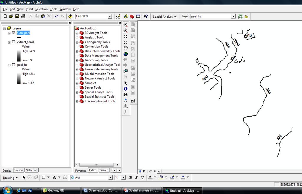
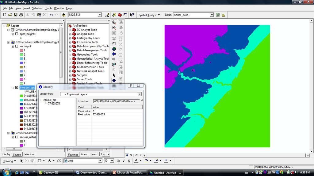
15 Key GIS analysis Data Conversion (select command to exclude the very low and high values from data ) Rasterization of Vector data (Available data was in the vector format so before the actual analysis the data was rasterized because the analysis is only possible with raster data) Raster Interpolation (The spot height map was interpolated to convert from point to continuous raster) Euclidean Distance command (The Road and Landmark map were first calculated by Euclidean Distace spatial analysis tool. With this tool we create a buffer of 250m and 200m to meet the specified criteria ) Raster Classification (Continuous (floating point) rasters must be reclassified as integer before they can be used. Generally, the values of continuous rasters are grouped into ranges, such as for height, or Euclidean distance outputs as in case of Road and Landmarks. Before the final analysis all the map are classified into one uniform criteria so that the overlay analysis can be done) Standardization In order to convert all the reclassified data into one unit it become standardized. A number of different standardization methods are available. In this case study the raw score was divided by maximum score to standardized. Overlay analysis by map single map algebra method

16 Table showing classification and Standardization of Different data layers Criteria Binary Raster Data Set Land use Fields Score Standardization Weight % Influence Residential 0 Park Land 0 Not available 0 Special 0 Purpose Land Institutional 0 Land Other Land 0 Farm Land 0 CA Land 0 Commercial 0 Land Industrial Land 1 Vacant Land 1 Reclassification (Grouping) Of landuse classes into 0 & 1 30

17 Ordinal Populat ion Continuous population data converted into Point density with pop field and 100 meter circle distance Standardized by dividing density layer by maximum value in single out put map algebra 50 Ordinal Spot Data The Raster cell values Standardized the raster cell values by dividing maximum value in single out put map algebra 20 Binary Reclassification into 0 & 1 0 Parcels Binary Road Less than 250m 0 Reclassification into 0 & Landma Less than 200m 1 Reclassification into 0 & 1 0 Binary rk

18

19

20

21 Surface analysis Interpolation Visiting every location in a study area to measure the height, magnitude, or concentration of a phenomenon is often difficult or expensive. Instead, you can measure the phenomenon at strategically dispersed sample locations and create a continuous surface by predicting values for all other locations. Input points can be either randomly or regularly spaced or based on some sampling scheme. ArcGIS Spatial Analyst provides inverse distance weighted (IDW), kriging, and spline interpolation, as well as polynomial trend and natural neighbor methods, which can be used to estimate elevation, rainfall, temperature, chemical dispersion, or other spatially continuous phenomena.

22 ArcGIS Spatial Analyst can also create nontraditional surfaces using various other functions. These include the ability to derive a density surface showing the density of objects, such as number of people per square kilometer; distance-based surfaces showing distance to various features, such as retail stores; and other surfaces. Using the derived surfaces, users can then directly display this new data, such as elevation from a terrain surface, or color-coded density areas for crime analysis. The inverse distance weighted and spline methods are referred to as deterministic interpolation methods because they assign values to locations based on the surrounding measured values. A second family of interpolation methods consists of geostatistical methods such as kriging, which are based on statistical models that include autocorrelation, the statistical relationship among the measured points. These geostatistical techniques not only have the capability to produce a prediction surface but also provide some measure of the certainty or accuracy of the predictions.

23 Spatial Interpolation Point Based Interpolation

24 Spatial Interpolation is.. Estimation of a z value for the surface at an unsampled location from a set of z values observed on surrounding points. (Locations on the surface at which measurements have been made) It is the observation that points close together in space are more likely to have similar values than points far apart (Tobler's Law of Geography)

25 Point Based Interpolation Methods Exact (quantitative interpolation) Methods Approximate Method Exact (quantitative interpolation) Methods 1. Proximal / Nearest Neighbour 2. B-Spline 3. Kriging Approximate Method 1. Inverse Distance Weighted

26 Point Based Interpolation Methods Exact (quantitative interpolation) Methods 1. Proximal Interpolation/ Nearest Neighbour Method Assumes the value at each grid cell location is the same as the value at the nearest observation Uses concept of thiessen polygons Thiessen polygons are defined around each observation. Only one observation is contained in each polygon. The boundaries of the polygon are MIDWAY between each neighbouring observation

27 Example of Thiessen polygons:

28 Point Based Interpolation Methods Exact (quantitative interpolation) Methods 2. B-Spline Method uses a piecewise polynomial to provide a series of patches resulting in a surface that has continuous first and second derivatives ensures continuity in: elevation (zero-order continuity) - surface has no cliffs slope (first-order continuity) - slopes do not change abruptly, there are no kinks in contours curvature (second order continuity) - minimum curvature is achieved produces a continuous surface with minimum curvature output data structure is points on a raster note that maxima and minima do not necessarily occur at the data points is a local interpolator

29 B-Spline method can be approximated by smoothing contours drawn through a TIN model

30 Point Based Interpolation Methods Exact (quantitative interpolation) Methods 2. B-Spline Method Advantages: best for showing very smooth surfaces can be exact or used to smooth surfaces Disadvantages: poor for surfaces which show marked fluctuations, this can cause wild oscillations in the spline

31 Point Based Interpolation Methods Exact (quantitative interpolation) Methods 3. Kriging Method developed by Georges Matheron, as the "theory of regionalized variables", and D.G. Krige as an optimal method of interpolation for use in the mining industry Kriging is a stochastic technique similar to inverse distance weighted averaging in that it uses a linear combination of weights at known points to estimate the value at an unknown point. Kriging uses a semivariogram, a measure of spatial correlation between two points, so the weights change according to the spatial arrangement of the samples. Unlike other estimation procedures investigated, kriging provides a measure of the error or uncertainty of the estimated surface

32 Kriging example:

33 Point Based Interpolation Methods Approximate Method Inverse Distance Weighted Interpolation Method: The value at each grid cell location is a DISTANCE-WEIGHTED AVERAGE of values located at nearby observations. It averages the values of sample data points in the vicinity of each cell and the closer a point is to the center of the cell being estimated, the more influence (weight) is has. It is a deterministic estimation, where values at unsampled points are determined by a linear combination of values at known sampled points It assumes that values closer to the unsampled location are more representative of the value to be estimated than samples further away

34 Distance-Weighted Interpolation DeMers, Fundamentals of Geographic Information Systems (2nd Ed). New York: Wiley.

35 IDW example: Copyright 1998 Helena Mitasova, GMS Laboratory, University of Illinois at Urbana-Champaign, currently at MEAS NCSU, Raleigh, NC,

36 Point Based Interpolation Methods Approximate Method Inverse Distance Weighted Interpolation Method: Advantages: Results in a smooth and continuous surface that changes between observations eg. Climatic data Derived surface passes through observed values Disadvantages: Requires subjective selection of parameters Does not interpolate beyond min and max values

37 Five Steps to Spatial Interpolation 1. Define purpose for interpolation 2. Define neighbourhood 3. Find points in neighbourhood 4. Choose mathematical function 5. Evaluate function for unknown points **steps are looped for every cell in the grid (not just one)

38

39

40

41

42 Summary Type of Interpolation Inverse Distance Weight Spline Regularized and Tension Kriging Classification Exact, Local, Deterministic Exact, Local Deterministic Local Stochastic When to use: To get fast results To get optimal results without much effort To get the best general results for more advanced analyses and visualization

43 Visual Comparison of DEMs Using Different Interpolation Methods Location: Lake of Bled in the western Slovenia IDW Spline Kriging Source:

44 Surface Analysis Using ArcGIS Spatial Analyst, users can build and analyze complex surfaces to identify patterns or features within the data. Many patterns that are not readily apparent in the original data can be derived from the existing surface. These include shaded relief, contours, angle of slope, aspect, and hillshade. These topographic derivatives give you the power to effectively relate your data to real-world terrain and analyze how variations in the topography will affect the problem in question.

45

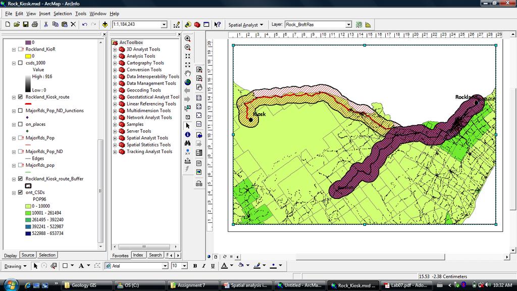
46

47

48 Contours Another but more simplistic ways of presenting terrain data is through contours Rasters Polylines Contours are lines that connect points of equal value (such as elevation, temperature, precipitation, pollution, or atmospheric pressure).

49 Contours The example below shows an input elevation grid and the output contour map. The areas where the contours are closer together indicate the steeper locations.

50 Surfaces from DEMs

51 Distance Analysis ArcGIS Spatial Analyst provides several distance mapping tools for measuring straight-line (Euclidean) distance and distance measured in terms of other factors such as slope, current road infrastructure, and land use. Calculating the accumulated cost of traveling, or mapping distance, can provide the user with additional data with which to make decisions. For example, the accumulated least cost of travel to a number of processing mills can be calculated while taking into consideration obstacles to travel. Road and waterway costs can then be assigned to restrict travel. Euclidean distance and cost distance are two main ways to perform distance analysis in ArcGIS Spatial Analyst. The Euclidean distance functions measure straight-line distance from each cell to the closest source. Not only can you determine allocation, but you can also calculate the distance and direction to the closest source.

52 Using the cost distance functions, you can create distance and direction rasters and compute the least-cost or shortest path from a chosen destination to your source point. The path distance functions add additional factors beyond the cost surface to account for actual travel distance over the terrain. This map shows the least-cost path between a stand of forest and the nearest sawmill. Factors such as slope, road infrastructure, and land use were combined with travel cost to find the optimal route

53 You can perform distance analysis in ArcGIS Spatial Analyst using two main methods: Euclidean distance and cost distance. The Euclidean Distance tool measures straight-line distance from each cell to the closest source; the source identifies the objects of interest, such as wells, roads, or a school. The distance is measured from cell center to cell center. Not only can you determine the distance each cell is to the closest source, you can calculate for each cell the direction and determine which source is the closest. The Cost Distance tool (or cost-weighted distance) modifies Euclidean distance by equating distance as a cost factor, which is the cost to travel through any given cell. For example, it may be shorter to climb over the mountain to the destination, but it is faster to walk around it. The Cost Allocation tool identifies the nearest (or least costly) source cell based on accumulated travel cost. The Cost Direction tool provides a road map, identifying the route to take from any cell, along the least cost-path, back to the nearest source.

54 Objectives: This lab will introduce you to the network problems of minimum routes. We will examine the minimum travel distance, time and population exposure for moving hazardous materials along Ontario roads. Software Environment: ArcGIS 9.2, Network Analyst, Spatial Analyst Data: 1. Major Roads of Eastern Ontario 2. Places in Ontario 3. Ontario Census Subdivisions (CSDs) 4. Province of Ontario /on_prov.shp 5. GRID of Ontario CSDs 6. Population Density GRID

55

56

57

58

59 Density Analysis The density function distributes a measured quantity of an input point layer throughout a landscape to produce a continuous surface. Available density mapping tools include Kernel Density Line Density Point Density Performing density analysis with ArcGIS Spatial Analyst.

60 By calculating density, you can create a continuous density surface from a set of input features. It can provide a more realistic interpretation of your values point values are spread out, giving you a better indication as to their distribution over a surface. Point Density calculates the density of point features around each output raster cell. Conceptually, a neighborhood is defined around each raster cell center, and the number of points that fall within the neighborhood is totaled and divided by the area of the neighborhood. Line Density calculates the density of linear features in the neighborhood of each output raster cell. Density is calculated in units of length per unit of area. Conceptually, a circle is drawn around each raster cell center using the search radius. The length of the portion of each line that falls within the circle is multiplied by its Population field value. These figures are summed and the total is divided by the circle's area. The figure below illustrates this concept:

61

62

63 Kernel Density calculates the density of point features around each output raster cell.

64

65 Map Algebra ArcGIS Spatial Analyst includes advanced map algebra functions for combining multiple maps, performing suitability analyses, assigning weights, and identifying relationships. Map algebra provides an easy-to-use and powerful way to define geographic analyses as algebraic expressions. This allows users to take their real-world data and apply algebraic functions to derive new results. For example, a single expression can be constructed to find the combined value of two datasets: >[(Raster1) + (Raster2)] These algebraic expressions can be simple arithmetic expressions or can consist of complex spatial and algebraic functions.

66 You can build complex expressions and process them as a single command. For example, you can use a single expression to find all the cells within a specific elevation range, apply a unit conversion such as feet to meters, and calculate the slope at each of those cells. Such an expression might look like the following: >=Elev_meters=Elev_feet*3.2808= Rain_total=Rain_April+Rain_May+Rain_June This graphic illustrates how mathematical operators and functions can be used to combine data on a cell-by-cell basis to derive new information.

67

68

69

70

71

72

73

74

75

76

77 12/30/2009 Extraction in ArcGIS

78 12/30/2009

79 12/30/2009

80 12/30/2009

81 12/30/2009

82 12/30/2009

83 12/30/2009

84 12/30/2009

85 12/30/2009

86 12/30/2009

87 12/30/2009

88 12/30/2009

89 12/30/2009

90 12/30/2009

91 12/30/2009

92 12/30/2009

93 12/30/2009

94 12/30/2009

95

96

97

98

99

100

101

102

103

104

105

106

107 Creating surfaces from points Surfaces of continuous data are usually generated from samples taken at points across the area. - ie: the irregularly spaced weather stations in a region can be used to create raster surfaces of temperature or air pressure. The resulting surface is a regular grid of values.

108 Creating Raster Surfaces Better Data = Better Grids More sample points More accurate measurements More appropriately distributed = better surface model

109 Creating Raster Surfaces Interpolation predicts values for cells in a raster from a limited number of sample data points. It can be used to predict unknown values for any geographic point data: elevation, rainfall, chemical concentrations, noise levels, and so on. Interpolation assumes that spatially distributed objects are spatially correlated.

110 Creating Raster Surfaces Why Interpolate? Visiting every location in a study area to measure the height, magnitude, or concentration of a phenomenon is usually difficult or expensive. Instead, dispersed sample input point locations can be selected and a predicted value can be assigned to all other locations. Input points can be either randomly, strategically, or regularly spaced points containing height, concentration, or magnitude measurements.

111 Creating Raster Surfaces A typical use for point interpolation is to create an elevation surface from a set of sample measurements. The resulting grid is a prediction of what the elevation is at any location on the actual surface.

112 Spatial Interpolation Most GIS packages come with a number of interpolation methods. Classifications of interpolations are: Exact or Approximate Local or Global Gradual or Abrupt Stochastic or Deterministic

113 Creating Raster Surfaces Exact Interpolator Interpolation surface agrees with original data values Approximate (Inexact) Interpolator Algorithm does not force the grid to honour the original data points

114 Creating Raster Surfaces Exact vs Approximate Interpolation If data is believed to have random error or uncertainty, use an inexact interpolator If data is believed to be absolutely accurate, and would be identical upon replication, use an Exact Interpolator In a sense, using an inexact interpolator shows a mistrust in the data, while using an exact interpolator shows a mistrust in the algorithm

115 Creating Raster Surfaces Global: methods apply a single mathematical function to all observed points and generally produce a smooth surface a change in one input value affects the entire map Local: methods apply a single mathematical function to small subsets of the total set of observed points and then link these regionally to create a composite surface covering the whole study area a change in an input value only affects the result within the window

116 Gradual: Gradual methods produce a smooth surface between sample points Abrupt: Creating Raster Surfaces Abrupt methods produce surfaces with a stepped appearance Terrain models may use both methods to visualize rolling terrain versus cliffs, ridges or valleys

117 Stochastic or Deterministic Stochastic: stochastic methods incorporate the random variation Deterministic: Used when sufficient knowledge about the geographical surface being modelled

118 Creating Raster Surfaces The best interpolation methods to use depends on: Objectives of the study (type of surface you are trying to generate) Ease of generating surface versus accuracy of the developed surface (the type of surface you are trying to model) The data (distribution of sample points)

119 Creating Raster Surfaces Basic Interpolation Methods Inverse Distance Weighted Spline Kriging

120 Inverse Distance Weighting IDW is a function that estimates cell values by averaging the surronding sample data points to each cell IDW assumes that each input point has a local influence that diminishes with distance. It weighs the points closer to the data source than those further away

121 In IDW, the predictive influence (weight) of a measured value depends on its distance from the prediction location. The strength of the dependency can be adjusted. IDW

122 IDW A higher weighting factor results in less influence from distance points Distance-weighted average preserves sample data values, and is therefore an exact interpolation technique IDW is very fast but has the tendency to generate bull s eyes Simple to use, very fast and provides reasonable results

123 Spline Instead of averaging values, like IDW does, the Spline interpolation method fits a flexible surface, as if it were stretching a rubber sheet across all the known point values. Useful if interested in estimated values that are below the minimum or above the maximum values found in the sample data. This makes the Spline interpolation method good for estimating lows and highs where they are not included in the sample data.

124 Spline Regularized Curved, more smooth and may not stay true to the sample points More elastic The higher the weight value, the smoother the grid Tension flatter therefore forcing the estimates to stay closer to the sample data. More rigid The higher the weight the coarser the surface

125 Spline This method is best for gently varying surfaces such as elevation, water table heights or pollution concentrations It is not appropriate if there are large changes in the surface within a short horizontal distance, because it can overshoot estimated values

126 Kriging Kriging is a multistep process Similar to IDS because it uses a linear combination of weights at known points to estimate the value of the grid. Assumes that the distance or direction between sample points reflects a spatial correlation that can be used to explain variation in the surface. Kriging fits a mathematical function to a specified number of points, or all points within a specified radius, to determine the output value for each location. Works best with data sets which have regions of densely scattered data and regions of lightly scattered data Kriging preserves sample data values (exact interpolator)