Textured RepTile Backlight

Transcription

1 Requirements Models: None Properties: None Editions: TracePro Expert Introduction There are a number of optical systems that use small, repeated optical geometry to perform. Examples include the structure for backlights, brightness enhancement films, and lenslet arrays. RepTile within TracePro allows repetitive structure to be placed on planar surfaces in a number of different patterns without the need to develop each one of the geometry elements. This not only saves time during the development phase, but also time during the ray trace analysis since the computation of intercepts with the RepTile geometry is computed analytically rather than through intersections with geometry. RepTile till now (i.e., prior to Version 4.0 of TracePro) has three cases: Constant: the RepTile geometry (e.g., sphere radius) is constant over the Tiles (or cells) that extend across the RepTile boundary, Variable Rows: the RepTile geometry (e.g., sphere radius) can vary as a function of the row number over the Tiles (or cells) that extend across the RepTile boundary, and Parameterized: the RepTile geometry (e.g., sphere radius) can vary as a function of both the row and column numbers over the Tiles (or cells) that extend across the RepTile boundary. All three of these make a single piece of geometry (e.g., a sphere) within a Tile (or cell) that has both a width and height assigned to it. The cases allow more control of the variation of the geometry as one goes down the bulleted list. However, in all cases the RepTile geometry, in a sense, is deterministic, meaning there is no ability to have a random array of RepTile geometry, multiple RepTiles per cell, and/or more complex parameterizations for the placement and shape of the RepTiles. The development of backlights for LCD displays is typically based on proprietary and often complex algorithms. These types of backlights are getting larger and more complex to ensure transfer efficiency to the viewer while maintaining illuminance uniformity over a prescribed range of angles. The rigorous demands of optical performance enforce a sizable amount of desired control of the luminance function of the backlight. Simply said, the three previously described methods may be too limiting for the development of large, complex, state-of-the-art backlit LCD displays. A new tool that allows the TracePro user to call upon previous designs that incorporate tailored structure that can be applied to surfaces in a backlit display are required. This new tool is called Textured RepTile. Textured RepTile allows the user to import a RepTile property from a text file. This text file includes the type of RepTile geometry, the parameters for describing each of the RepTile features, positioning of each feature, and the orientation of the feature (i.e., hole or bump). In Version 4.0 of TracePro, this new RepTile method is introduced, and in its initial implementation it is limited to the Sphere RepTile geometry. The remainder of this tutorial discusses how to create, import, apply, and ray trace a Textured RepTile that is applied to a backlight for a LCD. A constant pattern Texture pattern is applied to the back surface of the backlight, while a single cold cathode fluorescent lamp (CCFL) and injector reflector are used. This model provides the first iteration in the development of a Textured RepTile backlight the user must optimize the performance of it separately. Optimized performance implies a uniform luminance distribution over a prescribed set of angles (e.g., ±45 ). In the next section, the development of the backlight is discussed. In the third section, the development of the Texture is presented. Finally, in the last section the ray-trace results are given. Page 1 Copyright 2007 Lambda Research Corporation. All Rights Reserved.

2 Backlight Geometry A backlight for an LCD is at first level made of the following components: A thin sheet of plastic, such as acrylic, on which the back surface has structure placed. A reflective coating can be added on three of the four edges, while the remaining thin edge is at worst bare (i.e., anti-reflection coatings could be placed here). A reflector is placed on the one bare edge such that it runs the length of the plastic backlight. This reflector is some type of conic, such as circular, elliptical, or parabolic. Its output aperture is matched to the size of the bare edge of the plastic. A CCFL of small diameter is placed within the reflector. Positioning of the CCFL is typically not critical except for its absorption of rays re-incident upon it. A highly reflective diffuser is placed below the plastic backlight. The bottom of the backlight is the surface on which the Texture is placed. Finally, an observation plane is placed just above the output surface of the backlight plastic. The output surface is the one opposite of the Textured surface. There are a multitude of additional items that can be included in the model, including, brightness enhancement films, a wedge on the plastic backlight, the liquid crystal elements, additional diffusers, and the packaging around the backlight. For the purposes of this tutorial, we will simplify the development to only include the elements listed in the bulleted list above. Optimization of the system would include additional elements, structure, and optical properties. The purpose is to show how to implement Textured RepTile, and leave the optimization of the backlight to the user for their desired application. For the remainder of this tutorial, the following terms are used: Backlight = the thin sheet of plastic, Injector = the reflector that injects the light into the plastic, CCFL = the source placed within the injector, Feature = the individual spheres that are within the Texture file, Textures = the complete set of Features comprised by the Texture file, Diffuser = the highly reflective diffuser placed below the Textured surface of the backlight, and Screen = the surface on which we sample the output distribution from the backlight, where the term Observation indicates the surface on which we do this sampling. Page 2

3 Creating the Backlight We first create a square acrylic backlight with dimensions of 100 mm x 100 mm x 5 mm (XYZ). This solid is centered along the z direction. Figure 1 shows the dialog, Insert>Primitive Solid >Block, for this structure. We retain, at this time, the default bare surfaces on the two large surfaces and the edge in the +y direction. As shown in Fig. 2, for the three remaining surfaces we place the Mirror Surface property within the Default Catalog. Here are the steps for the process described here: 1. Open a New model window, 2. Select Insert>Primitive Solid >Block, 3. Enter the values as shown in Fig. 1, 4. Select Insert from the dialog, 5. Rescale the model window by first selecting the backlight and then View>Zoom>Selection, 6. Select Backlight Surfaces 2, 3, and 5 with CTRL left clicks, 7. Right click on one of these three surfaces and select Properties from the pop-up menu, or select the icon, 8. Select the Surface tab, 9. Enter the parameters as shown in Fig. 2, 10. Select Apply from the dialog, 11. Select the Material tab, 12. Enter the parameters as shown in Fig. 3, 13. Select Apply from the dialog, 14. You can Close the open dialogs, but it is not necessary, 15. Rename Surface 1 to Texture. To do this select it twice with a left click. When a rectangle appears around its current name, enter the new name. This is the surface on which we will later apply the Texture File, and 16. As per Fig. 4, inspect the System Tree such that the properties for Backlight are as shown (Note: Fig. 4 also shows all of the other objects that we will define in this section.) Page 3

4 Figure 1. Parameters to Insert the Backlight. Figure 2. Apply properties for Mirror application. Figure 3. Apply properties for the Backlight Material. Page 4

5 Figure 4. System Tree results for the surfaces of Backlight (except Texture). Page 5

6 Creating the Injector We will now create the reflector called the Injector, which injects all of the emitted rays into the backlight. The steps for doing this are: Select Insert>Reflector >Trough(Cylinder), Enter the values as shown in Fig. 5, Select Insert from the dialog, Select Insert>Primitive Solid >Block, Enter the values as shown in Fig. 6, Select Insert>Primitive Solid >Block, Enter the values as shown in Fig. 6, but set X: to and Name: to Endcap2, With CTRL left clicks, first select Injector, then the two End Caps, Select Edit>Boolean>Unite, Rescale the model window by first selecting Injector and then View>Zoom>Selection, Select all Injector surfaces or the Injector object, Right click on one of the selected objects or surfaces and select Properties from the pop-up menu, or select the icon, Select the Surface tab, Enter the parameters as shown in Fig. 7, Select Apply from the dialog, You can Close the open dialogs, but it is not necessary, and As per Fig. 8, inspect the System Tree such that the properties for Injector are as shown (Note: Fig. 8 also shows all of the other objects that we will define in this section.) Page 6

7 Textred RepTile Backlight Figure 6. Parameters to Insert the 2 Endcaps. Figure 5. Parameters to Insert the Backlight. Figure 7. Apply properties for Mirror application. Page 7

8 Figure 8. System Tree examples for the surfaces of the injector. Page 8

9 Creating the CCFL We will now create the source called the CCFL, which is a tubular fluorescent lamp. The steps for doing this are: 1. Select Insert>Primitive Solid >Cylinder/Cone, 2. Enter the values as shown in Fig. 9, 3. Select Insert from the dialog, 4. Rescale the model window by first selecting CCFL and then View>Zoom>Selection, 5. Select all CCFL surfaces or the CCFL object, 6. Right click on one of the selected objects or surfaces and select Properties from the pop-up menu, or select the icon, 7. Select the Surface tab, 8. Enter the parameters as shown in Fig. 10, 9. Select Apply from the dialog, 10. Select Surface 0 of the CCFL, 11. Select the Surface Source tab, 12. Enter the parameters as shown in Fig. 11, 13. Select Apply from the dialog, 14. You can Close the open dialogs, but it is not necessary, and 15. As per Fig. 12, inspect the System Tree such that the properties for CCFL are as shown (Note: Fig. 12 also shows all of the other objects that we will define in this section.) Page 9

10 Figure 9. Parameters to Insert the CCFL. Figure 10. Apply properties for Fluor White. Figure 11. Setting the Surface Source Parameters for the CCFL. Page 10

11 Figure 12. System Tree for the surfaces of the CCFL. Page 11

12 Creating the Diffuser We will now create the Diffuser, which is placed below the Backlight>Texture surface. The steps for doing this are: 1. Select Insert>Primitive Solid >Block, 2. Enter the values as shown in Fig. 13, 3. Select Insert from the dialog, 4. Rescale the model window by first selecting Diffuser and then View>Zoom>Selection, 5. Select all Diffuser surfaces or the Diffuser object, 6. Right click on one of the selected objects or surfaces and select Properties from the pop-up menu, or select the icon, 7. Select the Surface tab, 8. Enter the parameters as shown in Fig. 14, 9. Select Apply from the dialog, 10. You can Close the open dialogs, but it is not necessary, and 11. As per Fig. 15, inspect the System Tree such that the properties for Diffuser are as shown (Note: Fig. 15 also shows all of the other objects that we will define in this section.) Figure 13. Parameters to Insert the Diffuser. Figure 14. Apply properties for Diffuse White. Page 12

13 Figure 15. System Tree for the surfaces of the Diffuser. Page 13

14 Creating the Screen We will now create the Screen, which is placed above the Backlight>Surface 0 surface. The steps for doing this are: 1. Select Insert>Primitive Solid >Block, 2. Enter the values as shown in Fig. 16, 3. Select Insert from the dialog, 4. Rescale the model window by first selecting Diffuser and then View>Zoom>Selection, 5. Select all Screen surfaces or the Screen object, 6. Right click on one of the selected objects or surfaces and select Properties from the pop-up menu, or select the Apply Properties icon. 7. Select the Surface tab, 8. Enter the parameters as shown in Fig. 17, 9. Select Apply from the dialog, 10. Select Surface 1 of the Screen twice with left clicks, 11. Rename Observation, 12. Select the Exit Surface tab, 13. Enter the parameters as shown in Fig. 18, 14. Select Apply from the dialog, 15. You can Close the open dialogs, but it is not necessary, and 16. As per Fig. 19, inspect the System Tree such that the properties for Screen are as shown (Note: Fig. 19 also shows all of the other objects that we will define in this section.) Page 14

15 Figure 16. Parameters to Insert the Screen. Figure 17. Apply properties for Perfect Absorber. Figure 18. Setting of Exit Surface for Screen > Observation. Page15

16 Figure 19. System Tree for the surfaces of the Screen. You have now completed the geometry, except for the setup and designation of the Textured RepTile surface on the Backlight>Texture surface. In the next section we describe how to do this. Page 16

17 Setup and Application of the Textured RepTile There are two steps to this process: creation of the Textured RepTile property and application of the Textured RepTile to a planar surface. Each of these steps is described in the following sections. Creating the Textured RepTile Property We will now create the Textured RepTile Property, which is placed on the Backlight>Texture surface. The steps for doing this are: 1. Select Define>Edit Property Data >RepTile Properties, 2. Select Add Property (in the desired Catalog) in the left-hand part of the RepTile Editor (see Fig. 22), 3. Enter the data as shown in Fig. 20, 4. Left click on OK, 5. Select the browse button ( ) to the right of the File: line in the upper part of the RepTile Editor (see Fig. 22), 6. From the Open dialog (Fig. 21), navigate to the location of TextureTest1, 7. Select it and left click on Open, 8. Enter the Def. Width and Def. Height parameters as shown in Fig Click on Save and click OK on the confirmation dialog. 10. Exit the RepTile Editor. Figure 20. Enter New RepTile Property dialog. Figure 21. Open Texture File dialog. Page 17

18 Figure 22. The final RepTile Property Editor for TextureTest1 Property. Page 18

19 Applying the Textured RepTile Property We will now apply the Textured RepTile Property, which is placed on the Backlight>Texture surface. The steps for doing this are: 1. Select the surface Backlight>Texture as defined in Step 12 of Creating the Backlight, 2. Right click on Backlight>Texture and select Properties from the pop-up menu, or select the Apply Properties icon. 3. Select the RepTile tab, 4. Enter the parameters as shown in Fig. 23, 5. Select Apply from the dialog, 6. You can Close the open dialogs, but it is not necessary, and 7. As per Fig. 24, inspect the System Tree such that the properties for Backlight are as shown (Note: Fig. 24 also shows all of the other objects.) Figure 23. Apply TextureTest1 to the Backlight > Texture surface. Page 19

20 Figure 24. System Tree for the Backlight > Texture surface. You have now completed all aspects of the setup of the geometry and optical properties for this tutorial. In the next and final section, we discuss the setup of the Raytrace Options and the actual ray tracing and analysis. It is also a good time (if you have not been doing so already) to save your model. In this example, we have named the OML to be Backlight_TextureTest1.oml. Page 20

21 Raytrace Setup and Analysis There are two steps to this section: setup of the raytrace and the actual raytrace and analysis. Each of these steps is described in the following sections. Raytrace Options We will now setup the raytrace using Raytrace Options. Note that most of the data entered below are factory defaults for the parameters. Reset them as provided in Fig. 25 if you have Set Defaults in the past: 1. Select Analysis>Raytrace Options, 2. Select the Options tab, 3. Enter the parameters as shown in Fig. 25a, 4. Select Apply from the dialog, 5. Select the Wavelengths tab, 6. Enter the parameters as shown in Fig. 25b, 7. Select Apply from the dialog, 8. Select the Thresholds tab, 9. Enter the parameters as shown in Fig. 25c, 10. Select Apply from the dialog, 11. You can Close the open dialogs, but it is not necessary, and 12. Select Analysis>Simulation Mode. Figure 25. Raytrace Options... setup (a) Options, (b) Wavelengths, and (c) Thresholds. Page 21

22 Raytrace and Analysis We are now ready to do the raytrace and then analyze the results: 1. Verify that the source is setup correctly by selecting the Source tab at the bottom of the System Tree, 2. Expand the Surface sources item in the list (see Fig. 26), 3. Double click on CCFL/Source 0, 4. Verify that the resulting dialog (as within Fig. 26) agrees with that of Fig. 11, 5. Close the Apply Properties dialog, 6. Select Analysis>Trace Rays, 7. Ensure that the resulting dialog is as per Fig. 27, 8. Click Trace Rays, 9. Click on Yes within the Simulation Mode confirmation dialog, 10. The ray may take some time dependent on the speed of your computer, what else you are doing on the computer, and so forth. You can Cancel the ray trace and reduce the number of rays, if you desire to look at the results sooner, 11. Upon completion of the ray trace, select Screen>Observation from the Model System Tree, 12. Select Analysis>Irradiance/Illuminance Map, 13. Right click in the resulting Irradiance/Illuminance Map window, and select Irradiance/Illuminance Options or select from the menus Analysis>Irradiance/Illuminance Options, 14. Set the values within this dialog as shown in Fig. 28, 15. Click on Apply, 16. Figure 29 shows the resulting illuminance distribution for this model, 17. Select Analysis>Candela Plots>Rectangular Iso-Candela, 18. Right click in the resulting Rectangular Iso-Candela Map window, and select Candela Options or select from the menus Analysis>Candela Options, 19. Set the values within the two shown tabs of the dialog as per Fig. 30, 20. 2Click on Apply within each tab of the Candela Options dialog, and 21. Figure 31 shows the resulting intensity distribution for this model. Note that the illuminance distribution (Fig. 29) shows a lack of uniformity across the output surface. Most of the light is emitted toward the CCFL end of the display. The intensity distribution (Fig. 31) shows that most of the rays are emitted in the negative y direction, but the intensity distribution is much more uniform than that of the illuminance. One also desires to make the intensity distribution as uniform over the angular view range (±45 in this case). It is up to you to improve upon performance! This is accomplished by: Changing the radii, heights, and positions of the Features such that their density increases further away from the CCFL, Changing from Bump to Hole Features, Placing a wedge on the Backlight such that it thins further away from the CCFL, and Many other methods and techniques. As an example consider Figs. 32 and 33, which show the illuminance and intensity distributions, respectively, for a Textured hole array rather than a Textured bump array. The parameters for the Features are the same as for that of the results shown in Figs. 29 and 31. Note that the illuminance distribution (Fig. 32) has improved, while the intensity distribution (Fig. 33) has gotten a little worse. These figures address bullet 2 in the previous list. By adjusting the other items, especially the Feature density and sizes in the Texture file you can drastically improve performance. Page 22

23 Figure 26. Final verification that the source is correctly defined. You can click on Calculate Power to get the Power (lm) in the table to be set correctly. Page 23

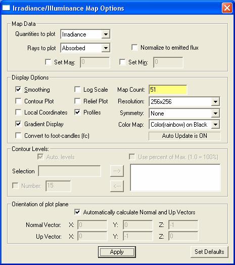
24 Figure 27. Trace Rays dialog. Figure 28. Irradiance/Illumination Map Options dialog. Page 24

25 Figure 29. Resulting illuminance distribution for the Backlight system. Figure 30. Two tabs from the Candela Options dialog. Page 25

26 Figure 31. Resulting intensity distribution for the Backlight system. Figure 32. Resulting illuminance distribution for the Backlight system using Holes instead of bumps. Page 26

27 Figure 33. Resulting intensity distribution for the Backlight system using Holes instead of bumps. Page 27